
学习在海马中产生正交的状态机
作者:Spruston, Nelson
主要的
智力以其核心表现出有机体或代理人动态互动,解释信息,适应不熟悉情况并执行复杂任务的能力。自然和人工智能研究中的一个核心概念是内部模型的概念。这些模型将外部世界的观察转换为组织良好的表示,从而实现了适应性行为。在神经科学中,内部模型的一个显着例子是认知图的概念。认知图是在20世纪初的概念化,是神经结构,使动物能够理解其环境并了解其身体与外部世界之间的相互作用,即使在新的情况下也支持有效的导航2。这个概念通过在海马中发现了细胞,在环境中特定位置有选择性地发射的神经元,这一概念获得了动力3,,,,4。从那以后,对认知图的神经基础进行了广泛的研究,揭示了有关神经元的发射特性的广泛知识,这些神经元包括啮齿动物的大脑5,灵长类动物(包括人类)6和其他动物7,,,,8。
这些基础研究表明,海马不仅捕获了环境的特征,还捕获了它们之间的关系以及动物中动物的作用。例如,许多海马神经元以活动形式携带的信息在环境中的特定位置(细胞的位置场)最大。3,而其他人不仅存储有关位置的信息,还存储有关上下文特征(例如运动方向)的信息9,,,,10,跑步速度9或运动历史11,,,,12,,,,13动物。海马神经元还可以学会代表更多抽象的空间,例如声音景观中的位置14,积累的证据15,概念,对象或事件之间的任意关系16和其他非空间维度17,,,,18。尽管关于构成海马认知图的神经元发射特性的知识广泛,以及有关其算法结构的最新想法19,,,,20,,,,21,,,,22,我们仍然尚未充分表征在中等复杂的任务的整个学习阶段的认知图。获取此类经验数据至关重要,技术进步(例如增加记录的神经元数量和纵向跟踪的持续时间)可以促进我们研究代表需要广泛探索和学习的复杂关系的认知图的形成的能力。在这里,我们利用这种技术进步来遵循每只老鼠数千个海马神经元中的神经活动,稳定多天或几周,因为他们学会了执行一项任务,要求它们形成代表空间,时间和抽象关系的认知图,同时与一位互动复杂但可预测的环境。
我们的结果表明,在学习过程中,小鼠通过一系列刻板的行为变化进行,这些变化反映了神经活动的结构化变化。具体而言,海马活动经历了一系列的去相关步骤,这些步骤使感觉刺激相似但潜在的任务状态不同的环境区域中的神经活动正交。我们分析了任务的代表性结构,可视化神经活动的低维几何形状,并将海马中的神经活动与各种认知模型和受过任务训练的人工神经网络中的单位活动进行了比较。我们表明,海马活动的日常动态与状态机的形成是一致的,该机器由任务状态的正交的潜在表示组成。这些潜在状态之间的过渡,每个编码特定的任务特征或段的每个编码,以预测动物与环境的相互作用的动力学。正交状态可以代表学习方面的类似感觉刺激,从而强调潜在任务结构是状态正交化的驱动力。
我们表明,可以通过多种计算模型复制在海马中观察到的最终正交状态机(OSM)表示,包括一种称为克隆结构性因果图(CSCG)的隐藏Markov模型(HMM)类型。21,,,,23以及某些复发性神经网络(RNN)。尽管各种模型可以通过特定的建筑设计或学习目标来实现最终的正交表示,但CSCG独特地复制了在动物中观察到的终端和逐步学习轨迹。CSCG学习动力与海马活动模式之间的这种一致性表明,在CSCG中实施的潜在国家推理过程可能是了解海马学习和认知图的形成原理的基础。相比之下,尽管它们在序列建模方面有效,但流行模型,例如长期记忆(LSTM)24或变压器25不要自然产生反映动物学习过程中观察到的表示的表示。我们进一步证明,神经活动在改变的任务条件下显示了OSM的灵活适应性,例如引入新的视觉提示和轨道段长度的调整。总而言之,这些发现阐明了有关认知图的形成的计算原则,并为未来人造系统的设计提供了潜在的指南。
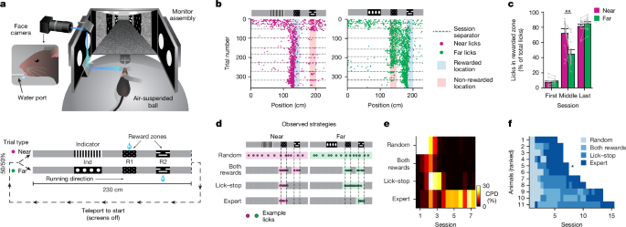
学习两种提示延迟选择任务
我们训练了在海马神经元中表达GCAMP6F的转基因小鼠,以在虚拟现实环境中导航,同时固定在头部以实现神经活动的成像,因为它们在两个线性轨道中学习了视觉提示与未来的水奖励交付位置之间的关系(图。1a;看 方法有关详细信息)。在每个试验中,水是在赛道开头或远处的两个奖励区之一中输送的,我们分别称为R1和R2。在这些奖励的位置之前,视觉上不同的指示提示(IND)完美地预测了奖励的位置(图。1a,底部和补充视频 1)。有效地执行此两种提示延迟选择(2ACDC)任务需要小鼠形成和使用长期记忆,以对指示器提示和奖励位置之间的关系以及指示提示的短期记忆之后的短期记忆它消失了,在奖励地点之前。

,虚拟现实行为设置(顶部)和任务的图表(底部)的图。虚拟现实行为设置的图是由J. Kuhl创建的。b,示例在近距离(洋红色)和FAR(绿色)试验类型的范围内的单个小鼠的舔图案。每个点代表一个试验中的单个舔,虚线表示每日会话之间的分离。c,在第一届会议的近距离试验类型,中级会议以及小鼠表现出专家表现(n= 11只小鼠;**p= 0.004,双面配对的学生t-测试;条形图显示平均值。d,说明小鼠在学习过程中表现出的四种不同行为策略。彩色阴影表示在基础函数内的非零区域,以回归,以抗跨轨道位置的舔密度。e,针对一个示例鼠标的四种行为策略的部分确定系数(CPD)。f,所有小鼠在会议上的主要策略(通过学习速度排名)。星号表示所示的鼠标e。值中的值e,,,,f通过将每个会话分成相等的持续时间(开始和结尾)的两个部分来计算。对于每个策略的会话数量(平均±s.e.m。),1.9±0.7(随机),2.0±2.5(均为奖励),3.3 -±2.8(Lick -Stop)和3.6±0.5(专家)。
最初对小鼠进行5天(每天1小时的一次)训练,以在球形跑步机上进行,并在黑暗中收集随机输送的水奖励。随后,打开屏幕以显示虚拟现实环境。在随后的每次1-H每日课程中,小鼠进行了大约80次200次试验(124次±43个试验,,n= 11只小鼠),奖励位置取决于试验类型。近似试验类型均以随机方式依次呈现(方法)。要开始一项新的试验,老鼠必须跑到走廊的尽头,这是由砖墙提示装饰的,而2-S的深色屏幕(Teleportation”)之前下一个审判。两种试验类型在指标区域以外的所有位置都具有相同的视觉提示。在指示区域和奖励区域之外,虚拟走廊的墙壁上装饰着相对毫无特色的灰色木纹(灰色区域)。在试验中(四个灰色区域)和整个试验(视觉上相同的灰色区域和奖励区提示)中的这种感觉歧义是任务的关键特征。在训练的前1届训练中,即使小鼠没有舔在奖励区域,也能提供水奖励,直到观察到持续的预期舔。在随后的所有日子里,只有在任何试验中,只有在正确的奖励区舔时就会在任何试验中奖励一滴水。在其他位置舔不罚款。因此,老鼠通过探索学习了任务,大概只有在预期奖励时才有动力放慢脚步和舔。
我们通过绘制舔行为作为在2ACDC任务的几天培训中所有试验的位置来评估学习的函数(图。1B)。最初,老鼠在整个赛道上舔了舔,但是他们很快学会了将两种试验类型的两个奖励区附近的曲目舔舔脚的部分。行为的这种变化发生在所有小鼠的2届会议中(扩展数据图。1a)。大约在同一时间,老鼠制定了一种中间策略,并在获得奖励后学会了抑制舔。结果,舔行为几乎是近试验类型的最佳选择(不是在远奖励区域舔),但对于远的试验类型仍然是最佳的(图。1C,中级会议),因为舔开始在近奖励区域,并且经常维持直到在遥远奖励区的奖励交付为止。通过额外的训练,小鼠最终学会了抑制远距离试验类型的近奖励区域中舔的舔,从而在两种试验类型上都取得了接近最佳性能(图。1C,上一次会话)。因此,舔行为似乎是通过逐渐变化的阶段演变而来的,其特征在于随着时间的流逝而改变的主要行为策略(图。1d):(1)随机舔,(2)在两个奖励地点舔,(3)在收集奖励后舔奖励位置并停止舔(舔lick -Stopâ),(4)仅舔接近正确的奖励地点(专家)。这些策略代表了逐渐出现和淡出的主要行为,而不是离散的,突然的变化。
我们使用了一种称为部分确定系数的统计方法来评估四种行为策略对小鼠整体行为的贡献。使用这四种行为策略作为回归剂,占所有会议中舔行为方差差异的3.5%(n=每只鼠标的9±3个会话)。该解释的差异百分比在涉及复杂任务的行为研究的预期范围内26。通过一次删除与每个行为策略一号对应的回归器,我们能够确定其对行为的独特贡献。部分确定分析的系数表明,这四种策略在学习过程中在不同点的连续波中占主导地位(图。1e),这是通过小鼠运行速度的曲线变化反映的(扩展数据图。1B)。尽管不同小鼠达到专家表现所需的会话数量有所不同,但通过这些主要的行为策略的逐渐发展始终观察到(图。1f)。
学习过程中海马活动的成像
在训练之前,将所有小鼠植入一个颅窗,以使用在背侧海马的CA1区域CA1中表达的GCAMP6F对神经活动进行成像(图。2a和 方法)。使用两光子随机访问介质对活动进行成像27。3毫米的颅窗很容易与具有5毫米视野的两光片随机访问介质对介质进行成像。数千个单元格(在一次会话中:4,682±827平均每只鼠标的平均范围:3,813 6,490;最大单个会话单元计数:5,545±848 – 848平均每只鼠标,范围:4,266 7,309;n= 11只小鼠)主要在视野中心附近,在每次训练和成像的几周内都很容易解决和重新识别(在跨疗程中跟踪的细胞:3,954± -平均每只动物的661范围:3,034 5,354;方法, 如图。2b并扩展数据图。2和3)。

,CA1成像植入物的图。CA1成像植入物的图是使用生物器创建的(https://biorender.com)。b,示例视野,细胞分割和提取的荧光信号。青色虚线标志着单个扫描条纹之间的边界。在所有11只小鼠中都观察到类似的成像和分割质量。c,在代表性小鼠中,近距离试验和远距离试验的试验平均神经活动与轨道位置(图7中的小鼠7。1f)。显示了按照指示试验类型(顶部)和相反试验类型(底部)排序的最大位置场质量中心的细胞。虚线标记指标和奖励提示的边界。d,类似于c,但在同一鼠标的第9节中。e,近乎交流的人口载体(PV)沿轨道位置的互相关矩阵在同一示例小鼠的第1、2、3、4和9的轨道位置。f,跨会话的互相关矩阵的不同区域的PV相关性,用于脱离灰色区域的相关性(灰色),PRE-R2区域(浅蓝色),Pre-R1区域(深蓝色),初始区域(红色),指示区域(橙色)和末端区域(青色)为每只小鼠显示,并在所有小鼠中平均。矩阵中的虚线标记指示器和奖励提示的边界。曲线代表平均值,阴影表示S.E.M.比较所有会话显示Pre-R1和Pre-R2区域之间的显着差异(双面Wilcoxon签名式测试,***p= 9.96 - 105,来自11只小鼠的97个会议)。第一个和上一个会话之间的比较表明,PER-R2,PRE-R1,指标(减少)和初始区域(增加; ***)发生了显着变化。p<0.001;n= 11只小鼠)。对于非对抗区域,观察到相关性显着下降(**p= 0.002;n= 11只小鼠)。末端区域的变化不显着(NS)。g,在五个课程中学习的神经歧管的3D UMAP和状态图,以及同一示例鼠标e,选择2D视图以最好地说明3D结构捕获的学习动力学。1a显示)(显示cf)用于图形的可读性。源数据
根据峰活动的位置进行订购细胞,发现在两种试验类型的整个虚拟轨道上都有明显分解的空间响应对角线带(图。2C)。根据相对试验类型的空间活性模式对细胞进行订购也显示了对角线空间条带,表明在两种试验类型中,许多细胞在相似位置都活跃。然而,在指标提示位置,试验类型之间的活性差异最大(图。2C),表明感觉信息在这个早期学习阶段主导了神经活动。实际上,在四个灰色区域之一中最活跃的细胞在其他灰色区域也显示出中等活性(图。2C)。我们观察到跨小鼠的任务的初始表示,有很大的个人变异性,其中一些从一开始就显示出强烈的去相关性,而另一些则显示出很高的相关性(扩展数据图。4)。经过几天的训练,这些2ACDC任务的这些基于神经活动的地图在单个试验类型(在几个灰色区域中)以及两种试验类型的相应位置之间越来越区分(图。2d)。
学习过程中有系统的海马变化
通过计算两种试验类型的种群矢量相关性,比较了近距离试验类型的代表性结构(方法),在训练期间在选定的位置中系统地减少。对轨道所有区域的近距离试验类型之间的互相关分析表明,指示器提示区域的相关性较低,如该位置的视觉刺激差异所预期的那样(图。2e,f)。无论是在试验类型内外,轨道的四个灰色区域在大多数小鼠的第一节中都适度相关,但是到第三次疗程,相关性大大降低了(图。2e,f并扩展数据图。5显示种群矢量角度也接近90°),这表明海马对这些视觉上相似区域的表示形式正交。跨试验类型的相应位置之间的相关性以有序的方式降低,在远奖励区(pre-r2)前,在轨道区域的神经活动通常比接近奖励区之前的区域早(pre-r1;图;图。2e,f)。与指标提示相对应的神经活动,同时已经从发作中显示出低相关性,随着暴露于两种试验类型的增加而进一步脱离相关(图。2e,f)。尽管大多数轨道区域都将完全去相关成近乎正交表示,但在大多数小鼠的整个训练中,轨道的开头和结尾保持相关性(扩展数据图。4)。这表明去相关过程是由任务结构塑造的,因为在收集奖励之后,动物缺乏有关下一个试验类型的信息,直到看到下一个指标。
总之,这些结果揭示了海马学会如何代表任务结构的系统进步。最初,海马在单个线性轨道内的四个视觉上相似的灰色区域中的每个区域中的每个区域都区分了,这表明海马首先学习了任务环境的顺序性质。通过额外的培训,在两种试验类型的相应位置进行的神经活动逐渐被脱字,通常是从奖励之前的区域开始,然后是接近奖励之前的区域。尽管视觉线索相同,但仍会向正交化的这种渐进性去相关,这表明出现了不同的任务状态表示。这种神经活动中的逐渐去相关与小鼠的舔行为逐渐发展(扩展数据图)共同发展。6)。这种平均学习轨迹(图。2f在大多数单个小鼠中观察到)(例如,图。2e);但是,在神经活动和行为中都发生动物对动物的变异性表明,某些动物的学习方式可能有所不同(图。1f并扩展数据图。4)。
海马OSM代表
我们进一步可视化了使用非线性维度降低技术,特别是均匀的歧管近似和投影(UMAP)的神经活动的日常动力学。28。使用单个嵌入空间来减少数千个单元的活性到低维(3D)UMAP空间中的点,使用纵向注册的数据收集到整个成像的纵向注册数据,其中每个点代表了所有单元的活性单成像框架(图。2G和方法)。值得注意的是,这种UMAP表示不仅呼应了我们先前描述的逐渐去相关和正交化(图。2e,f并扩展数据图。4和5),但这也使我们能够直观地观察学习过程中神经歧管的总体拓扑变化。
在这里,我们描述了来自代表性鼠标的UMAP,该鼠标展示了所有学习阶段。初始会话的UMAP表示形式明显地聚集了与每个感觉提示相关的神经活动。尽管有这种区别,但在此阶段,总体神经歧管似乎相对非结构化(图。2G,阶段0)。到第二天,UMAP采用了轮毂和辐条的外观(图。2G,第1阶段),与所有灰色区域相对应,与灰色区域和所有其他线索之间的活动轨迹相对应(即指示提示,近距离奖励提示以及深色传送区域)。该结构暗示,与线性轨迹概念相关的神经活动可能在这一点上尚未完全发展。在奖励区嵌入附近的另一个散射点云对应于水回报的时期和守回后的时期,在此期间,小鼠未运行。到第三次会议,UMAP采用了一个类似环的结构,该结构在2-S的深色传送期间被活动封闭,该结构与一个试验结束和下一次试验的开始联系在一起(图。2G,第2阶段)。随着训练的进行,两种试验类型的活动轨迹变得越来越鲜明,最终类似于分裂的结婚戒指,由一支乐队组成,该乐队分为两块,中间有钻石。在这里,分裂谱带对应于鼠标运行时神经活动的主要歧管,而钻石对应于小鼠静止时的点云,大部分是在奖励消耗期间和之后。我们推测,在UMAP表示中可以观察到的这种奖励相关点云可能与神经活动的重播有关,并且可能有助于海马及其下游目标的突触可塑性29(扩展数据图。7和补充视频 2显示单次试验UMAP动力学)。分裂环UMAP的逐渐外观反映了上述试验型去相关的动力学(图。2e,f)。
相关矩阵和UMAP都反映出的表示结构的观察到的渐进性变化类似于逐渐发展的状态机,经过了几个有意义的中间阶段,并最终达到了捕获任务本质的结构(图。1a,底部和图。2G,在UMAPS下方的状态图)。这个学习过程涉及在人口活动水平上两种试验类型的不同区域的相似感觉输入的几个阶段,最终为任务的先前潜在状态产生正交状态表示。在这种学识渊博的结构中,指标线索的短期记忆是通过代表不同潜在状态的不同神经活动来实现的。我们称此任务的学会表示为OSM。
OSM形成过程中的单细胞调整变化
海马中神经表示的正交化反映了在学习过程中动物行为的变化以及动物行为的变化而发生的单个神经元的发射特性的变化。随着培训的进行,神经元在调整属性中会经历修改,从而变得更有选择性和响应与任务相关的功能。
在学习的早期阶段观察到的一个重大变化是最初调整为多个灰色区域为更具选择性细胞的神经元的转化,在更少甚至一个灰色区域发射(图。3a)。随着学习的继续,神经元在近距离试验类型中表现出越来越不同的调整,尤其是在奖励前轨道区域(PER-R1和PRE-R2)。这包括最初的沉默神经元,这些神经元在一种试验类型而不是另一种试验类型的特定区域中变得活跃,以及最初在两种试验类型上都活跃的神经元,但最终通过减少其他试验类型的活动而成为特定的试验类型(图。3b,c)。这些分离器细胞11,,,,12在整个学习过程中出现(图。2e和3)。

,在第1阶段2过渡期间(前三个会话;顶部)的四个示例细胞调整为灰色区域的四个示例细胞的位置调整,以及在近试验中,灰色区域调节细胞的空间分散指数的累积百分比,第1节。相对于第3节(底部;绘图显示平均值±S.E.M.p<16;n= 11只小鼠)。b,在九个会话中进行近9个疗程的近距离试验的会话平均活性(顶部),以及的累积百分比f/f调谐细胞的试验类型之间的前R2差异,会议1对9(底部;图显示平均值±s.e.m.p0<16;n= 11只小鼠)。c,类似于b对于Pre-R1区域(图显示平均值±S.E.M.,***p<16;n= 11只小鼠)。d,相关系数与差分评分散射图的活性超过2 s.d。高于专家会议中的平均值。这x轴表示接近远的相关系数,并且y轴表示差分d= |一个_nearâ一个_far |/max(一个_靠近,一个_far),其中 一个_ near和一个_FAR是近距离试验中的峰值神经活动。根据图中的相对位置手动选择示例细胞并颜色编码。eg,近(洋红色)和FAR(绿色)试验的试验平均调谐曲线,例如d,通过调谐表型标记。h,散点图(左)显示了在初始或末端区域(灰色),指示区域(红色)以及奖励或奖励前区域(CYAN)中最大程度调整的细胞的学习进展(新手,中级和专家),并归一化每个小鼠的密度图(右)针对每个轨道段调整的人群。我,跨训练(按相关分类= 2,差异得分= -0.5阈值;n= 11只小鼠)。j,在专家阶段沿轨道区域的响应类型的分布(平均值±S.E.M。;n= 11只小鼠)。近距离试验的轨道图(类似于图。1a显示)(显示一个c,,,,h)用于图形的可读性。源数据
为了进一步表征专家阶段中单个细胞的各种调谐特性,对于每个细胞,我们计算了一个差异评分,该分数量化了近距离试验类型之间峰活动的分数差异,并将其与两种响应之间的相关性绘制(
如图。3D)。这两个特征将单元的调整响应分为直观类别。具有较大差异的细胞表现出强烈的分离响应,显示出试验类型之间的调谐幅度差异很大(例如,图。3e,蓝色1和蓝色2,以及无花果。3f,红色1和红色2)。差异得分低和高相关系数的细胞表现出响应,在两种试验类型中都显示出相似的调整(例如,图。3e,蓝色4)。相比之下,差异较低和低相关系数的细胞表现出分离器响应的重新映射,其调谐峰具有相似的幅度,但在近距离试验中发生在不同位置。图中心的细胞表现出中间表型。例如,某些细胞显示位置和分离器表型的组合(例如,图。3f,红色4)。两种特征的中心中心的细胞都表明,位置细胞和分离器细胞之间的区别最好被描述为具有多种调谐特性的响应的连续体。此外,这些响应特性是塑性的,学习可能反映了这些不断变化的神经元反应。
我们通过根据细胞的最大调整位置分离这些响应类型而不是学习的出现:试验开始和结束,指标区域以及奖励或奖励前区域(图。3H, 左边)。Plotting their positions in the difference score versus correlation scatter plot for novice, intermediate and expert sessions revealed gradual changes across learning for each group.Track start or track end responses were initially concentrated near the moderately high correlation and low-to-intermediate difference score region, suggesting variable but mostly correlated tuning.With learning, these cells quickly adopted more obvious place responses with very high correlations and low difference scores, consistent with the population correlation analysis showing high correlation at the trial start or trial end even in well-trained mice (Fig.2e–g)。Indicator-tuned cells transitioned from a scattered distribution to a concentrated density in the upper region with high difference scores, highlighting their rapid transformation into responses that more completely distinguished between different visual cues.By contrast, cells tuned to the reward and pre-reward regions gradually transitioned from place-like responses to splitter responses, indicating that these sensory-ambiguous regions require more prolonged learning to produce differential responses.
Quantifying the percentage of cells with responses in three arbitrarily defined regions of the scatter plot revealed a gradual increase in the percentage of splitter responses and a corresponding drop in the place-like responses during learning, whereas remapping splitter responses remained low (Fig.3i)。Although for simplicity we quantified responses in these categories, in reality they represent points on a continuum rather than discrete cell types.At the expert stage, cells with place and place-splitter responses dominated the track start and end regions, whereas cells with splitter and remapping splitter responses dominated the regions in the middle of the track (Fig.3J)。In summary, these single-cell tuning changes can be understood as the hippocampus learning to extract the latent task structure despite the ambiguity of immediate sensory experiences.To facilitate exploration of these diverse single-cell tuning properties, we developed an interactive visualization tool, which is available athttp://cognitivemap.janelia.org/。Hippocampal maps versus computational models
The large number of neurons that we recorded over many days of training presents a unique opportunity to probe the learning algorithms that lead to the gradual emergence and final representational structure of the 2ACDC task. Several recent theoretical models have conceptualized cognitive maps as learned internal models of the world that allow animals to predict upcoming sensory experiences from their understanding of the environment and their actions in it
20,,,,21。To test whether this class of models can provide insight into the measured hippocampal learning, we analysed an HMM-based model called the CSCG21,,,,23。Fundamentally, HMMs and CSCGs aim to uncover hidden structures from sequential data, capturing meaningful latent states and their temporal dependencies (Fig.4a)。CSCGs make use of ‘clones’ that assign states to fixed sensory observations via a deterministic emission matrix (Fig.4a,b)。State occupancy probabilities are influenced by current and past sensory stimuli, and the model was constructed by finding a transition matrix between states that best predicts sensory sequences using the Baum–Welch expectation maximization algorithm30(如图。4a, Extended Data Fig.8和方法)。

, HMM diagram showing latent states and transition probabilities with fixed emission probabilities.b, CSCG diagram with 100 clones per sensory symbol.c, Final transition graph of the CSCG trained on the 2ACDC task, showing distinct latent states and their sensory inputs. Coloured circles indicate specific track regions similar to Fig.2g。d, CSCG (top) and CA1 (bottom) cross-correlation matrices between near and far trials during learning (the CA1 data are the same as Fig.2e;sessions 1, 3, 4 and 9). Track diagrams for near and far trials (similar to Fig.1a) are shown for readability of the graphs.e, RNN diagram showing sensory input processing (x((t)) through recurrent units, which produce the hidden state y((t), to predict next input (\(\hat{X}\)((t + 1)).f,,,,g, Final correlation matrices for near versus far trial representations across models. Polynomial softmax uses 8th power normalization.h, Schematic showing how correlated high-dimensional activity (green and red vectors) can yield orthogonal outputs through readout projection (yellow plane).我, Mean final correlation matrix quantification across mice (n = 11) and models (independent simulations runs:n = 20 (CSCG),n = 10 (Hebbian-RNN),n = 42 (vanilla RNN exponential softmax),n = 47 (polynomial softmax),n = 10 (rectified linear (ReLU)),n = 10 (LSTM) andn = 10 (transformer); two-sided unpaired Student’st-tests with Bonferroni correction for multiple comparisons).j, Time for key regions to reach correlation threshold (0.3), normalized to training duration. Data from model runs (n = 18 (CSCG),n = 8 (Hebbian-RNN),n = 15 (vanilla RNN exponential softmax) andn = 39 (polynomial softmax)) and mice (n = 11 mice; two-sided paired Student’st-tests without correction for multiple comparisons). The bar graphs in我,,,,jshow mean ± s.e.m.;*p < 0.05, **p < 0.01 and ***p < 0.001.源数据The CSCG model recapitulated the final representation and learning trajectory of the hippocampus. Like the UMAP embedding of hippocampal activity (Fig.2g), the learned state transitions of the CSCG closely resembled the task architecture (Fig.4C), with trial-type-specific state sequences producing distinct sensory experiences on the two trial types (Fig.4C, upper and lower branches), and shared state sequences producing the sensory sequence shared across trials (Fig.4C, middle branch). We then compared clone occupancy probabilities to population vector activity in the hippocampus. We found that during training, the state probabilities gradually progressed through stages of orthogonalization that closely mirrored the dynamics that we observed in the hippocampus (Fig.4d并扩展数据图。8)。The ability of the CSCG model to recapitulate key features of hippocampal neural dynamics suggests that sequence-dependent extraction of latent states from potentially ambiguous or identical sensory inputs may represent a fundamental computational principle of hippocampal learning.
4e)。RNNs using rectified linear or sigmoid activation functions trained using backpropagation through time achieved high accuracy in predicting next sensory inputs without developing the orthogonalized representations characteristic of hippocampal activity (Fig.4fand Extended Data Fig.9)。In these models, activity corresponding to the same sensory inputs in different latent states remained highly correlated, contrasting sharply with our experimental observations in mice (Fig.4f,i)。This is because perfect task performance only requires that population neural activity be orthogonal in the low-dimensional task-relevant subspace that is read out for stimulus prediction, leaving many task-irrelevant dimensions that have no effect on task performance (Fig.4H)。Similarly, more complex neural network architectures widely used in sequence learning tasks, LSTM
24networks and transformers25achieved high prediction accuracy but did not naturally produce orthogonalized representations unless explicitly encouraged to learn the orthogonalized representations as part of their learning objective (Fig.4f,i并扩展数据图。9)。Conversely, RNNs with softmax activation functions did produce fully orthogonalized representations when fully trained, more closely resembling the hippocampal data (Fig.4g,i)。This shows that in addition to learning rules, the learning objective and the choice of architectural features critically influences the final representational structure of these networks.Biologically plausible neural network models and plasticity rules can also produce hippocampus-like representations. Previous work has suggested that spike-timing-dependent plasticity31,,,,32can stably encode sequences33in a manner that is robust to noise34。Spike-timing-dependent plasticity has also been shown theoretically to facilitate forming predictive maps35,,,,
36,,,,37and approximate HMM learning38。We thus built a spiking RNN model that included a soft winner-take-all (sWTA) mechanism, which leverages the principle of feedback inhibition to ensure that only the highest firing neurons remain active within the network.Using only a timing-based Hebbian plasticity rule based on local activity38(that is, no end-to-end training or explicit task), the model (Hebbian-RNN) learned orthogonalized representations of the 2ACDC task (Fig.4G并扩展数据图。10)。These findings underscore the ability of canonical, biologically plausible learning mechanisms to shape hippocampal representations and suggest that sWTA-like mechanisms help to promote decorrelated cognitive maps.Although the correlation values of the mice were slightly higher than those of the fully decorrelated models (Fig.4i), this difference may be attributed to ongoing learning processes in the mice at the time of measurement. In rapidly decorrelating regions such as the off-diagonal areas, mice showed near-complete decorrelation (Fig.2f)。Crucially, the specific decorrelation sequence observed during learning provided a stringent constraint on potential models of hippocampal function. In our experimental data, we observed an average pattern in which off-diagonal elements decorrelated first, followed by the pre-R2 region, and finally the pre-R1 region (Fig.2e,f)。Among the models tested, only the CSCG consistently reproduced this precise decorrelation trajectory (Fig.4d,j)。Other models that achieved decorrelated final states, including vanilla RNNs and Hebbian-RNNs, showed different sequences of decorrelation, with pre-R1 often decorrelating before or simultaneously with pre-R2 (Fig.
4J)。This distinction in learning dynamics provides a critical means of discriminating between potential algorithmic accounts of hippocampal function.It also suggests that the CSCG based on the Baum–Welch expectation maximization algorithm captures critical algorithmic properties of hippocampal learning that can inform future work to mechanistically explain cognitive map formation through biologically plausible plasticity rules.Although these results support the CSCG as a leading model, further research is needed to fully elucidate the complex mechanisms and principles contributing to cognitive map formation.Adaptation of the existing hippocampal state machineTo investigate whether and how the learned hippocampal state machine would adapt to novel task features, we expanded and modified the structure of the task. First, after mice learned the task with the original indicator cues (cue pair A), we replaced them with two unfamiliar visual patterns. To do this, we developed four unique indicator pairs (cue pairs B, C, D and E) and presented them to mice that had already learned the original cue pair (Fig.
5a
)。Every day, the mice were initially exposed to cue pair A for a duration of 5–10 min, after which the indicators for the task were replaced with one of the novel pairs.This change enabled us to collect neural activity data for both the original and the new cue pairs during the same session.Training on the new cue pair continued until the mouse could proficiently execute the task, demonstrated by restricting its licking to the rewarded location or just before it on 75% of the trials for three successive sessions.Mice were then sequentially trained on each subsequent novel indicator pair on the following days in the same manner.Through this training process, mice learned the new cue pairs in significantly fewer trials (147 ± 39 trials for the new cue pairs compared with 483 ± 70 trials for the original cue pair;n = 3 mice;*p < 0.05, unpaired Student’s t-测试;如图。5b)。

, Original and novel indicator pairs.b, Number of trials required to reach high performance (75% or more correct licking) for each indicator pair. For original indicators,n = 3 mice; for novel indicators,n = 11 training periods across the same 3 mice;*p = 0.039, two-sided unpaired Student’st-测试。The bar graphs show mean ± s.e.m.;the dots represent individual training periods.c, PV cross-correlation between the neural activity for trials with the original and new indicators for the same trial type (near (top left) and far (top right)), and between near and far trials for the new indicators (bottom left)。Quantification of the diagonal cross-correlations in three cross-correlation matrices (line and shading indicate mean ± s.e.m.;n = 3 mice) is also shown (bottom right).d, Conceptual diagram for the incorporation of new indicator states into an existing state machine.e, Place field locations in the stretched near trials plotted against those in the regular near trials (n = 3 mice, data pooled together). The histograms of field locations in the two stretched regions are plotted to the right (line and shading indicate mean ± s.e.m.;n = 3 mice).f, Similar toebut for the far trials. Track diagrams for near and far trials (similar to Fig.1a) have been added toc,,,,e,,,,f。源数据Comparing population vector correlations of the neural activity for trials with novel indicators versus the original indicators revealed high similarities in neural representations between the old and the new tasks in all track regions except the indicator region (Fig.5C
In other words, the neural activity in the presence of new indicators mirrored the common task structure while maintaining information about the visual identities of the novel indicator cues.In terms of the state machine framework, this suggests that once a state machine is established in the hippocampus, it can be effectively reused for new task variants.New task elements can be incorporated into the existing state machine, either through the creation of new states or linking new sensory inputs to existing states (Fig.5d)。This flexible adaptation and integration, in turn, expedite learning.
In a second variation of the task, we extended the length of the grey zones following the indicator cue and after the first reward cue, thus requiring animals to travel longer distances to reach the reward zones (Fig.5e,f和方法)。We inserted these ‘stretched trials’ after every 5–6 regular trials to evaluate how well-trained mice for the original task respond to the altered environment without extensive adjustment to these task modifications (方法)。In both stretched near (near′) and stretched far (far′) trial types, mice displayed a tendency to lick towards the beginning of the usual reward location, even though the reward cue was not yet encountered (Extended Data Fig.9)。A comparison of the tuning location for each cell during normal and stretched trials of the same type (that is, near–near′ or far–far′) provided insights into how the mice might perceive the modified task (Fig.5e,f)。As expected, place fields were tuned to similar locations in both regular and stretched trials for the initial, unmodified portion of the track.When mice entered the first stretched region in near trials, cells normally tuned to the grey region before the first reward (pre-R1) maintained their activity throughout the extended segment (Fig.5e;n = 3 mice). This potentially indicates that the animal may believe it remains in the same patch of the grey zone right before the first reward region. During far trials, the difference in reward location expectation produces a different pattern. When mice entered the first stretched region in far trials, neurons did not persistently extend their activity. Instead, they rapidly shifted their tuning to align with the region just before the second reward area (pre-R2), as if the mouse was anticipating the second reward location (Fig.5F)。However, when the mouse eventually saw the first reward cue, the representation quickly resets and anchors to the representation reflecting the first reward region.These results imply that, when the animals encounter modified components of the task, the neural representations can settle into discrete states to mirror inferred latent states under conditions of uncertainty (Fig.5e,f)。These discoveries substantiate the idea that the learned cognitive map exhibits the properties of a state machine that can infer and flexibly use learned states in novel situations.Investigating how various computational models respond to such task alterations presents an exciting avenue for future research39。
讨论
We assessed neural activity in a large population of neurons as mice learned a virtual reality task over the course of several days to weeks. Our findings reveal the gradual emergence of a cognitive map within the hippocampus, coinciding with improvements in task performance. This development is reflected in changes to both population-level neural activity and the response properties of individual neurons. Well-trained mice exhibit robust short-term and long-term memory — processes that are consistent with the structure of the mature cognitive map, including the ability to produce effective behaviour in novel environments with similar structure but altered features. The cognitive map has features of a state machine with orthogonalized representations of latent states that the animal must discover to perform the task efficiently and that meaningfully represent altered versions of the environment. Computational modelling suggests that many features of this OSM, including the gradual dynamics of its formation, share properties with a type of HMM called CSCG that is learned using the expectation maximization algorithm.
We further showed that RNNs can also produce orthogonalized representations under certain conditions. Vanilla RNNs trained with backpropagation through time can achieve orthogonalized representations when using sWTA activation functions such as softmax. In addition, biologically plausible spiking RNNs coupled with sWTA dynamics and trained using Hebbian plasticity are sufficient to construct the final OSM. This combination of RNN, sWTA and Hebbian plasticity has been previously shown to approximate HMM learning via expectation maximization38, highlighting that known biological mechanisms may construct graph-like representations of environments where animals repeatedly experience sequences of sensory stimuli, including rewards that are delivered in latent contexts. However, although these RNN models capture the final orthogonalized representations, the specific sequences of decorrelation do not match those observed in animals. In addition, we found that widely used sequence learning models in artificial intelligence, specifically LSTMs and transformers, trained to predict the next element in a sequence using backpropagation of error, do not naturally produce orthogonalized representations like those found in the mouse hippocampus. However, we found that this key property of the hippocampal OSM could be observed in LSTM when the cost function explicitly penalized activity correlation between the two trial types. Our modelling results suggest that the emergence of orthogonalized representations could be driven by specific architectural choices (such as activation functions) and cost functions rather than the learning algorithm alone. Our approach can be viewed as a feature-matching method for inferring learning rules from neural activity dynamics, complementing recent work on identifying learning rules from neural observables40,,,,41。
CSCG captures both the final representations and the learning trajectory observed in animals, strengthening its promise for modelling hippocampal function21,,,,23。The success of the CSCG compared with RNNs may be attributed to its training via Baum–Welch expectation maximization, its ability to decouple latent dynamics from observations and its use of discrete representations.These features make the CSCG particularly well suited for planning and reasoning in artificial intelligence systems, mirroring the role of the hippocampus in flexible behaviour.
这些结果对理解可能有助于海马认知图的形成的建筑特征,目标和可塑性机制具有重要意义。其中最重要的是,我们的建模表明,具有适当建筑选择的本地Hebbian学习和梯度下降学习都足以构建正交图。Hebbian plasticity does not require feedback from other brain areas, as it is determined entirely by the relative timing of presynaptic and postsynaptic spikes local to the modified synapse32。This is fundamentally different from the methods typically used to adjust synaptic weights in artificial neural networks, such as in vanilla RNNs, LSTMs and transformers, which rely on backpropagation of error through explicitly defined cost functions42。Nevertheless, there is good evidence that feedback-based plasticity is important in the hippocampus43,,,,44, and it has been proposed to be a key element in approximating the backpropagation of error algorithm in the brain45。涉及目标,错误或奖励信号的基于反馈的机制也可能是工具性的。这些机制可能与Hebbian可塑性一致,以构建认知图和/或通过选择性将信息从已建立的认知图与其他大脑区域进行选择,从而更参与精炼行为政策和其他特定于任务的功能。Our data indicate that task representations and behavioural policies based on them are formed in lockstep, as previously suggested46。A likely candidate mechanism for the contribution of synaptic plasticity during feedback is behavioural timescale synaptic plasticity43。未来的实验用新颖的感官提示代替奖励可以阐明是否需要奖励为提取潜在的任务结构或仅感官预测是否足够。这样的研究将在认知图形成中区分奖励驱动的学习和纯粹基于感觉的预测编码。除了这些生物学机制外,最近的机器学习进步还提供了有关通过返回流式过程实现去相关的新观点。Techniques such as contrastive losses47and object-centric representations48provide alternative approaches to generating decorrelated representations, which may have parallels in biological learning systems.
It is important to note that plasticity mechanisms in other brain regions probably contribute to our observations. For example, CA1 receives most of its excitatory synaptic input from CA3, where recurrent connections49, attractor dynamics50and Hebbian plasticity have all been observed51。Plasticity in CA3, as well as other brain regions, may thus result in changes in the firing of the pyramidal neurons that we imaged in CA1.Although our RNN models are not detailed representations of hippocampal circuitry, they can be considered as abstractions of CA3 function.Although we recorded from CA1, it is plausible that CA1 inherits orthogonalized representations from upstream regions such as CA3.We propose that the existence of multiple forms of synaptic plasticity across different brain regions allows unsupervised and supervised (and reinforcement) learning to work together to reduce sensory interference, build robust models of the environment and direct the content of these models to promote adaptive behaviours.Understanding how these diverse plasticity mechanisms interact to produce flexible and efficient cognitive maps remains a key challenge in understanding the computational principles of the brain.Future research should focus on elucidating the specific roles and interactions of Hebbian, feedback-based and other learning rules in cognitive map formation and utilization across different brain regions.Identifying the loci and molecular mechanisms of these processes will be crucial for advancing our understanding of how the brain learns and adapts to complex environments.
A classical concept in computer science, a finite state machine is a computational structure consisting of a finite set of states with the transitions between them based on defined inputs or conditions52。States reflect current sensory input from the environment and the body of the animal, as well as latent information such as the recent history of sequential observations.Transitions are constrained by the current state and neurally encoded transition probabilities, and determined by the movements of the animal and the sensory input it receives from the environment.We posit that neural activity in the hippocampal OSM could contribute to adaptive behaviour, such as speeding up, slowing down or licking53。These behaviours in turn influence neural activity, and thus transitions to new states in the hippocampal OSM, both by changing the external and internal sensory experience of the animal and by changing the stimuli coming from the environment.The hippocampal OSM operates in closed loop with the rest of the brain, the body of the animal and its environment to produce the properties of a state machine.
The emergence of the OSM involves dynamic changes in single-cell tuning properties, which we characterized using a novel 2D feature space. This approach reveals a continuum of response types rather than discrete categories, challenging traditional cell-type classifications and demonstrating that single-cell tuning, when properly interpreted in the context of a latent state inference20,,,,21,,,,23,,,,54, can provide valuable insights into learning dynamics at a fine granularity. We observed that individual neurons dynamically transition between functional roles as learning progresses, adapting their representations to capture task-relevant information. This flexibility suggests that hippocampal neurons act more like plastic state cells than rigid place or splitter cells. Plasticity of these features is responsible for the gradual discovery and representation of task-related latent states. Our findings extend beyond the concepts of splitter cells and pattern separation, showing that cognitive map formation is not a simple accumulation of these phenomena but a systematic, stereotypical progression in neural representations. Our findings support the long-standing proposal that sparse orthogonal representations are a powerful mechanism for memory and intelligence55,,,,56。
Our modelling efforts complement existing frameworks in hippocampal research by specifically addressing the dynamics of learning in ambiguous environments such as the 2ACDC task that we used here. We explored a range of models to capture the gradual emergence of orthogonalized representations observed in our data. This approach revealed that certain computational principles, particularly those involving latent state inference, are crucial for replicating both the final representations and the learning trajectory seen in animals. Although influential models such as successor representations19,,,,57and the Tolman–Eichenbaum machine20have provided valuable insights into cognitive maps, they focus on different aspects of hippocampal function. Successor representations efficiently compute long-term reward predictions by factoring the value function into state dynamics and reward but require pre-defined states. The Tolman–Eichenbaum machine emphasizes generalization of structural knowledge across environments and does not address how new latent states could be rapidly learned in new environments. Our work, similar in conceptualization to the CSCG21,,,,23, extends the field by providing data elucidating how the hippocampus learns de novo latent states and resolves perceptual ambiguity within a single environment, a process fundamental to the formation of precise cognitive maps.
Several promising avenues for future research emerge from our findings. Although our models capture key aspects of hippocampal representations, further work is needed to fully explain the specific sequence of orthogonalization observed in animals. Future models could incorporate additional biological mechanisms, such as replay29, to more accurately mirror the learning process. In addition, investigating the interaction between hippocampal and neocortical representations58during learning could provide valuable insights into how the brain forms and uses cognitive maps across different timescales and levels of abstraction.
In conclusion, our study provides a comprehensive view of cognitive map formation in the hippocampus during learning of a moderately complex task. The emergence of OSM representations offers a fundamental framework for understanding neural computation, memory and intelligence. Our findings reveal key principles underlying biological cognitive map formation, offering insights that could both deepen our understanding of adaptive behaviour and guide the development of more sophisticated artificial intelligence systems with robust world models.
方法
All procedures were performed in accordance with the Janelia Research Campus Institutional Animal Care and Use Committee guidelines. Both male and female GCaMP6f (Thy1-GCaMP6f59) transgenic mice were used, 3–6 months of age at the time of surgery (3–8 months of age at the beginning of imaging studies).
外科手术
Mice were anaesthetized with 1.5–2.0% isoflurane. A craniotomy on the right hemisphere was performed, centred at 1.8 mm anteroposterior and 2.0 mm mediolateral from the bregma using a 3-mm diameter trephine drill bit. The overlying cortex of the dorsal hippocampus was then gently aspirated with a 25-gauge blunt-tip needle under cold saline. A 3-mm glass coverslip previously attached to a stainless-steel cannula using optical glue was implanted over the dorsal CA1 region. The upper part of the cannula and a custom titanium headbar were finally secured to the skull with dental cement. Mice were allowed to recover for a minimum of 2 days before being put under water restriction (1.0–1.5 ml daily), in a reversed dark–light cycle room (12-h light–dark cycle).
行为
Virtual reality setup
The virtual reality behavioural setup was based on a design previously described60。The spherical treadmill consisted of a hollowed-out Styrofoam ball (diameter of 16 inches, 65 g) air-suspended on a bed of 10 air-cushioned ping-pong balls in an acrylic frame.Mice were head fixed on top of the treadmill using a motorized holder (Zaber T-RSW60A; MOG-130-10 and MOZ-200-25, Optics Focus) with their eyes approximately 20 mm above the surface.To translate the movement of the treadmill into virtual reality, two cameras separated at 90° were focused on 4-mm2regions of the equator of the ball under infrared light60。Three axis movement of the ball was captured by comparing the movement between consecutive frames at 4 kHz and readout at 200 Hz (ref.60)。A stainless-steel tube (inner diameter of 0.046 inches), attached to a three-axis motorized stage assembly (Zaber NA11B30-T4A-MC03, TSB28E14, LSA25A-T4A and X-MCB2-KX15B), was positioned in front of the mouse’s mouth for delivery of water rewards.The mouse was shown a perspective corrected view of the virtual reality environment through three screens (LG LP097QX1 with Adafruit Qualia bare driver board) placed roughly 13 cm away from the animal (Fig.1a)。This screen assembly could be swivelled into position using a fixed support beam.All rendering, task logic and logging were handled by a custom software package called Gimbl (https://github.com/winnubstj/Gimbl) for the Unity game engine (https://unity.com/)。All inter-device communication was handled by a MQTT messaging broker hosted on the virtual reality computer.Synchronization of the virtual reality state with the calcium imaging was achieved by overlaying the frame trigger signal of the microscope with timing information from inbuild Unity frame event functions.
To observe the mouse during the task without blocking its field of view, we integrated a periscope design into the monitor assembly. Crucially, this included a 45° hot-mirror mounted at the base of a side monitor that passed through visible light but reflected infrared light (Edmund Optics 62-630). A camera (Flea3-FL3-U3-13Y3M) aimed at a secondary mirror on top of the monitor assembly could hereby image a clear side view of the face of the mouse. Using this camera, a custom Bonsai script61monitored the area around the tip of the lick port and detected licks of the mouse in real time that were used in the virtual reality task as described below.
Head fixation training
After recovering from surgery, mice were placed on water restriction (1.0–1.5 ml daily) for at least 2 weeks before behavioural training. Body weight and overall health indicators were checked every day to ensure mice remained healthy during the training process. Mice were acclimated to experimenter handling for 3 days by hand delivering water using a syringe. For the next three sessions, with the virtual reality screens turned off, mice were head fixed on the spherical treadmill while water was randomly dispensed from the lick port (10 ± 3 s interval; 5 µl per reward). These sessions lasted until mice acquired their daily allotment of water or until 1 h had passed. We observed that during this period most mice started to run on their own volition. Next, we linked water rewards to bouts of persistent running and increased this duration across sessions till the mouse would run for at least 2 s straight (approximately five sessions). During this time, we also slowly increased the height of the animal with respect to the treadmill surface across sessions to improve performance. Mice that did not show sufficient running behaviour to acquire their daily allotment of water were discarded in further experiments.
2ACDC task
At the beginning of each trial, mice were placed at the start of a virtual 230-cm corridor. The appearance of the walls was uniform except at the location of three visual cues that represented the indicator cue (40 cm long) and the two reward cues (near or far; 20 cm long). Depending on the trial type, a water reward (5 µl) could be obtained at either the near or far reward cue (near and far reward trials). The only visual signifier for the current trial type was the identity of the indicator cue at the start of the corridor. For the first 2–3 sessions, the mouse only had to run past the correct reward cue to trigger reward delivery (‘guided’ sessions). On all subsequent sessions, mice had to lick at the correct reward cue (‘operant’ sessions). No penalty was given for licking at the incorrect reward cue. In other words, if the mouse licked at the near reward cue during a far trial type, then the mouse could still receive a reward at the later far reward cue. Upon reaching the end of the corridor, the virtual reality screen would slowly dim to black, and mice would be teleported to the start of the corridor to begin the next semi-randomly chosen trial with a 2-s duration. The probability of each trial type was 50%, but to prevent bias formation caused by very long stretches of the same trial type, sets of near or far trials were interleaved with their number of repeats set by a random limited Poisson sampling (lambda = 0.7, max repeats = 3). The identity of the indicator cue was kept hidden for the first 20 cm of the trial and was rendered when the mice passed the 20-cm position. To internally track the learning progress of the mouse, we utilized a binarized accuracy score for each trial depending on whether the mouse only licked at the correct reward cue. Once the mouse had three sessions in which the average accuracy was above 75%, we considered the mouse to have learned that cue pair.
2ACDC task with novel indicators
For 3 mice out of the 11 well-trained mice on the original 2ACDC task, we subsequently trained them to perform the 2ACDC task novel indicator pairs. After reaching three consecutive sessions with more than 75% task accuracy for the original 2ACDC task, the novel task was introduced in the following session, but with the original task shown for the first 5–10 min at the beginning of each session before switching completely to the new task. When the mouse could perform the new task for 3 consecutive days with more than 75% accuracy, we moved on to the next novel indicator pair until the last one was finished (four novel indicator pairs in total).
2ACDC task with extended grey regions
As another modification to the original task design, the grey regions were extended in certain trials, which we called the ‘stretched trials’. In the stretched trials, the linear track was extended from 230 cm to 330 cm, and the reward positions were moved from [130, 150] cm to [180, 200] cm (the first rewarding (near) object), and [180, 200] cm to [280, 300] cm (the second rewarding (far) object). Note that the distance between the indicator cue and the near object in the stretch trial is equal to the one between the indicator cues and the far object in the normal trial. During a session with stretch trials, following a 5-min warm-up using only the normal 2ACDC trial, the stretch trial was adopted at intervals of every five or six trials.
Calcium imaging
Neural activity was recorded using a custom-made two-photon random access (2P-RAM) mesoscope27and data acquired through ScanImage software62, running on MATLAB 2021a. GCaMP6f was excited at 920 nm (Chameleon Ultra II, Coherent). Three adjacent regions of interest (each 650 µm wide) were used to image dorsal CA1 neurons. The size of the regions of interest was adjusted to ensure a scanning frequency at 10 Hz. Calcium imaging data were saved into tiff files and were processed using the Suite2p toolbox (https://www.suite2p.org/)。This included motion correction, cell regions of interest, neuropil correction and spike deconvolution as described elsewhere63。
Multiday alignment
To image the same cells across subsequent days, we utilized a combination of mechanical, optical and computational alignment steps (Extended Data Figs.2和3)。First, mice were head fixed using a motorized head bar holder (see above), allowing precise control along three axes (roll, pitch and height) with submicron precision.Coordinates were carefully chosen at the start of training to allow for unimpeded animal movement and reused across subsequent sessions.The 2P-RAM microscope was mounted on a motorized gantry, allowing for an additional three axis of alignment (anterior–posterior, medial–lateral and roll).Next, we utilized an optical alignment procedure consisting of a ‘guide’ LED light that was projected through the imaging path, reflected off the cannula cover glass and picked up by a separate CCD camera (Extended Data Fig.2b)。Using fine movement of both the microscope and the head bar, the location of the resulting intensity spot on the camera sensor could be used to ensure exact parallel alignment of the imaging plane with respect to the cover glass.
To correct for smaller shifts in the brain tissue across multiple sessions, we took a high-resolution referencez-stack at the start of the first imaging session (25 μm total, 1-μm interval; Extended Data Fig.2C)。The imaging plane on each subsequent session was then compared with this reference stack by calculating a cross-correlation in the frequency domain for each imaging stripe along all depth positions.By adjusting the scanning parameters on the remote focusing unit of the 2P-RAM microscope, we finely adjusted the tip or tilt angles of the imaging plane to achieve optimal alignment with the reference stack.We used a custom online Z-correction module (developed by Marius Pachitariu64, now in ScanImage), to correct forz和xydrift online during the recording within each session, using a newly acquiredz-stack for that specific session.
To find cells that could be consistently imaged across sessions, we first performed a post-hoc, non-rigid, image registration step using an averaged image of each imaging session (diffeomorphic demon registration; Python image registration toolkit) to remove smaller local deformations (扩展数据图。2g–i)。Next, we performed hierarchical clustering of detected cells across all sessions (Jaccard distance; Extended Data Fig.3)。Only putative cells that were detected in 50% of the imaging sessions were included for further consideration.We then generated a template consensus mask for each cell based on pixels that were associated with this cell on at least 50% of the sessions.These template masks were then backwards transformed to the spatial reference space of each imaging session to extract fluorescence traces using Suite2p.
数据分析
Coefficient of partial determination
To assess the unique contribution of each behavioural strategy (random licking, licking in both reward locations, lick–stop and expert) to overall animal behaviour, we used the coefficient of partial determination (CPD). In this analysis, a multivariable linear regression model was first fitted using all behavioural strategies as regressors, providing the sum of squares error (SSE) of the full model (SSEfullmodel)。Each regressor was then sequentially removed, the model refitted, and the SSE without that regressor (SSE〜我) was computed. The CPD for each regressor, denoted as CPD我, was then calculated as CPD我 = (SSE〜我 − SSEfullmodel)/SSE〜我, revealing the unique contribution of each behavioural strategy to the overall variance in licking behaviour.
Place field detection
To identify significant place cells, we utilized an approach based on Dombeck et al.65(but see also Grijseels et al.66for overall caveats with such approaches). Place fields were determined during active trials, indicated by active licking within reward zones, and at running speeds greater than 5 cm s−1。For detecting activity changes related to position, we first calculated the calcium signal by subtracting the fluorescence of each cell mask with the activity in the surrounding neuropil using Suite2p.Next, the baseline fluorescence activity for each cell was calculated by first applying Gaussian filter (5 s) followed by calculating the rolling max of the rolling min (‘maximin’ filter; see Suite2p documentation).This baseline fluorescence activity (f) was used to calculate the differential fluorescence (Δf0/f), defined as the difference between fluorescent and baseline activity divided byf0。Next, we identified the significant calcium transient event in each trace as events that started when fluorescence deviated 5σ from baseline and ended when it returned to within 1σ of baseline.0Here baseline σ was calculated by binning the fluorescent trace in short periods of 5 s and considering only frames with fluorescence in the lower 25th percentile.
Initially, putative place fields were identified by spatially binning the resulting Δf/f0activity (bin size of 5 cm) as continuous regions where all Δf/f0values exceeded 25% of the difference between the peak of the trial and the baseline 25th percentile Δf/f0值。We imposed additional criteria: the field width should be between 15 and 120 cm in virtual reality, the average Δf/f0inside the field should be at least four times greater than outside; and significant calcium transients should occur at least 20% of the time when the mouse was active within the field (see above). To verify that these putative place fields were not caused by spurious activity, we calculated a shuffled bootstrap distribution for each cell. Here we shuffled blocks of 10-s calcium activity with respect to the position of the mouse and repeated the same analysis procedure described above. By repeating this process 1,000 times per cell, we considered a cell to have a significant place field if putative place fields were detected in less than 5% of the shuffles.
Population vector analysis
For the analysis of similarity of representation between near versus far trial types, we performed population vector correlation on the fluorescence Δf/f数据。Each 5-cm spatial bin, we defined the population vector as the mean Δf0/fvalue for all neurons. Fluorescence data were included only when the speed of the mouse exceeded 5 cm s−10。The cross-correlation matrix was generated by calculating the Pearson correlation coefficient between all location pairs across the two trial types.空间分散指数
为了评估跨单个细胞的空间分散程度,例如区分单个位置与多个位置的区分,我们将单细胞调音曲线越过轨道位置并对其进行了归一化,以使曲线下的面积为1。
The spatial dispersion index is defined as the entropy of this normalized Δf/f0signal by: entropy = −∑ [p((我) × log2p ((我)], 在哪里p((我) denotes the probability associated with each position bin index.UMAP
To visually interpret the dynamics of high-dimensional neural activity during learning, we utilized UMAP on our deconvolved calcium imaging data. The UMAP model was parameterized with 100 nearest neighbours, three components for a three-dimensional representation, and a minimum distance of 0.1. The ‘correlation’ metric was used for distance calculation. The data, a multidimensional array representing the activity of thousands of cells concatenated from several imaging sessions, were fitted into a single UMAP model. This resulted in a three-dimensional embedding, in which each point characterized the activity of the neuron ensemble at a single imaging frame.
造型
CSCG
In the 2ACDC task, the combination of position along the track and trial type defines a state of the world (
z)。Although this state is not directly observable to the animal, it influences the sensory observation (x) that the animal perceives.环境中的状态顺序遵守马尔可夫特性,其中下一个状态的概率分布(即下一个位置和试验类型)仅取决于当前状态,而不是所有先前的状态,假设动物始终以固定速度行驶。当动物学习环境的结构并建造地图时,它试图学习哪种状态(位置,试验类型),遵循哪些状态以及它们产生的感官体验。这可以看作是马尔可夫学习问题。A HMM consists of a transition matrix whose elements constitute\(p({z}_{n+1}| {z}_{n})\)that is, the probability of going from statezn时间n到zn+1时间n + 1, an emission matrix whose elements constitute\(p({x}_{n}|{z}_{n})\), that is, the probability of observingxnwhen the hidden state iszn, and the initial probabilities of being in a particular hidden state\(p({z}_{1})\)。
The CSCG is an HMM with a structured emission matrix in which multiple hidden states, referred to as clones, deterministically map to the same observation.换句话说,\(p({x}_{n}=j|{z}_{n}=i)=0\)如果\(i\notin C(j)\)和\(p({x}_{n}=j|{z}_{n}=i)=1\)如果\(i\in C(j)\), 在哪里\(C(j)\)refers to the clones of observationj21(扩展数据图。8f)。The emission matrix is fixed and the CSCG learns the task structure by only modifying the transition probabilities (Extended Data Fig.8e,f), making the learning process more efficient. The Baum–Welch expectation maximization algorithm was used to update the transition probabilities such that it maximizes the probability of observing a given sequence of sensory observations67,,,,68,,,,69。
We trained the CSCG on sequences of discrete sensory symbols mimicking the sequence of patterns shown to the mice in the two tracks. Each 10-cm segment of the track was represented by a single sensory symbol. In addition, the teleportation region was represented by a distinct symbol repeated three times, spanning 30 cm. In the rewarded region, the mice could receive both visual input and a water reward simultaneously. However, our model could only process a single discrete stimulus at a time. Thus, we divided the rewarded region into two parts. We presented the visual cue first, mimicking the ability of the mouse to see the rewarded region ahead before reaching it. Subsequently, we presented a symbol representing the water stimulus, which was shared across the two trials. The near trial sequence, denoted as [1,1,1,1,1,1,2,2,2,2,1,1,1,4,6,1,1,1,5,5,1,1,7,0,0,0], and the far trial sequence, denoted as [1,1,1,1,1,1,3,3,3,3,1,1,1,4,4,1,1,1,5,6,1,1,7,0,0,0]′, were used. Where 1 represented the grey regions, 2 and 3 indicated the indicators for near and far tracks, respectively, 4 denoted the visual observation associated with the first reward zone, 5 represented the visual stimulus associated with the far reward zone, 6 denoted the common water reward received in both tracks, 7 represented the brick wall at the end of each trial, and 0 indicated the teleportation region (Extended Data Fig.8C)。However, the representations and learning dynamics are not sensitive to the addition of the brick wall and teleportation segments.
We initialized the model with 100 clones for each sensory observation symbol and performed 20 iterations of the expectation-maximization process at each training step with sequences from 20 randomly selected trials, comprising both near and far trial types. We extracted the transition matrix at different stages of learning and used the Viterbi training algorithm to refine the solution21, and then plotted the transition matrix as a graph, showing only the clones that were used in the representation of the two trials (Extended Data Fig.8a)。We ran multiple simulations and compared how correlation between the two trial types changed over learning for different positions along the track (Extended Data Fig.8b)。
We also explored alternate sequences of sensory stimuli. In one variant, we provided the water symbol before the visual symbol of the reward zone (for example, […1,1,1,6,4,1,1,1…] where 6 represented the water and 4 denoted the visual symbol). In addition, we introduced a symbol that conjunctively encoded the simultaneous water reward and visual symbol (for example, […111,4,6,111…] in the near trial and […111,5,8,111…] in the far trial, where 6 denoted a combined code for water and visual R1, and 8 represented a combined code for water and visual R2; Extended Data Fig.8C)。Although the final learned transition graphs matched for all the four sequence variants, the exact sequence of learning differed.Specifically, reward cue followed by a visual cue for reward zone often led to decorrelation of pre-R1 followed by pre-R2 (Extended Data Fig.8c,d), contrary to what is often observed during learning in animals.
香草Rnns
我们实施了自定义RNN模型来学习2ACDC任务的结构。Task sequences incorporated numerical symbols with unique meanings: ‘1’ denoted the grey region;‘2’ and ‘3’ represented near and far cues, respectively;‘4’ and ‘5’ indicated near and far reward cues, respectively;‘6’ symbolized reward;and ‘0’ denoted teleportation.近试验的一个例子遵循结构:1,1,1,1,1,1,2,2,2,2,2,1,1,1,1,4,4,6,1,1,1,5,5,1,1,0和远程试验遵循:1,1,1,1,1,1,3,3,3,3,3,3,1,1,1,4,4,4,1,1,1,5,6,1,1,0。我们将这些数值符号转换为一式式编码以表示这些类别。RNN由输入层,一个经常性的隐藏层和输出层组成。输入和输出层都包含七个单元,对应于任务中的唯一感觉提示。隐藏的层大小在200至5,000个单位之间变化,具体取决于特定变体。我们探索了隐藏层的四个激活函数:指数软max,relu,多项式软max和sigmoid。指数和多项式软马克斯函数实现了软冠军的全部机制,而relu和sigmoid提供了更多传统的激活模式。随着ADAM Optimizer的时间,使用反向传播对模型进行了训练。根据激活函数进行调整,学习率在0.002到0.2之间,以确保稳定的训练。我们使用跨透镜损失作为目标函数。For each simulation, we generated sequences of 40–100 trials (random mixture of near and far trials), with half used for training and half for testing.每个试验由23个时间步长组成,与虚拟轨道沿线的位置相对应。Models were trained for 60–1,200 epochs.我们进行了多个具有不同随机种子的独立模拟,以评估可变性,范围为4到48个模拟,具体取决于特定的模型变体。为了初始化模型,我们使用了从重量矩阵的正态分布中得出的小随机值。The input-to-hidden and hidden-to-hidden weight matrices were initialized with a standard deviation of 0.001, whereas the hidden-to-output weight matrix used a standard deviation of 0.01–1, depending on the model variant.
Hebbian-RNN
以前的工作38showed that a local Hebbian learning rule in a RNN can approximate an online version of HMM learning. We used an RNN consisting ofk = 100 recurrently connected neurons andn = 96 feedforward input neurons. The feedforward input neurons carried orthogonal inputs for each of the 8 sensory stimuli, with 12 different neurons firing for each stimulus. The recurrent weightsvand feedforward weightswwere initialized from a normal distribution with 0 mean and standard deviation 2.5 and 3.5, respectively. The membrane potential of thekth neuron at timet由\({u}_{k}^{t}={\sum }_{i}^{N}{w}_{{ki}}{x}_{i}^{t}+{\sum }_{j}^{K}{v}_{{kj}}\,{y}_{j}^{(t-\Delta t)}\), 在哪里wkiis the feedforward weight from input neuron我to RNN neuronk,,,,vKJis the recurrent weight from neuronjto neuronk, Δt = 1 ms is the update time, and\({x}_{i}^{t}\)和\({y}_{j}^{t-\Delta t}\)are exponentially filtered spike trains of the feedforward and recurrent neurons, respectively (exponential kernel time constant of 20 ms). The probability of neuronkfiring in Δtwas computed by exponentiating the membrane potential and normalizing it through a global inhibition,\({f}_{k}=\frac{{e}^{{u}_{k}}}{{\sum }_{l}^{K}{e}^{{u}_{l}}}\)。For each neuronk, spikes were generated with a probability offkby a Poisson process, with a refractory period of 10 ms during which the neuron cannot spike again. When the postsynaptic neuronkspiked, then the weights onto neuronkwere updated as\(\Delta {w}_{ki}(t)=\alpha ({e}^{-{w}_{ki}}{x}_{i}(t)-0.1)\)和\(\Delta {v}_{kj}(t)=\alpha ({e}^{-{v}_{kj}}{y}_{j}(t)-0.1)\), 在哪里αis the learning rate (0.1) and\({y}_{j}(t)\)is the exponentially filtered spike train. Both weightsv和wwere kept excitatory. We computed the correlation between the RNN representation of different positions in the near and far trial types at different stages during learning and compared it with the cross-correlation matrices for mice.LSTM我们使用与香草RNN相同的任务结构和输入序列实现了LSTM网络。The LSTM model consisted of a single LSTM layer with 500–1,200 hidden units, followed by a linear readout layer.输入和输出层都包含七个单元,对应于任务中的唯一感觉提示。LSTM处理了输入序列,并为每个时间步生成隐藏状态。这些隐藏的状态是分析的主要输出,也通过线性读数层来生成预测。我们探索了几种LSTM变体,包括标准模型,一个在隐藏状态上具有L1正则化的模型,另一个在隐藏状态上应用了辍学,一个具有相关性惩罚的版本,以鼓励在不同试验类型的隐藏状态之间进行脱字。These models were trained using the Adam optimizer with learning rates between 3 × 10
−4
and 5 × 10−4, using cross-entropy loss as objective function.Training proceeded for 200–300 epochs on sequences of 100 trials, with half used for training and half used for testing.我们用不同的随机种子进行了多个独立的模拟。对于所有LSTM变体,我们分析了隐藏状态动力学(某些变体的单元格状态),研究了它们在预测奖励位置时不同试验类型之间的相关结构以及模型的准确性。
变压器
We implemented a transformer architecture based on the minGPT repository (https://github.com/karpathy/minGPT), specifically using the GPT-micro configuration. This model uses 4 layers, 4 attention heads and an embedding dimension of 256. The transformer was adapted to learn the 2ACDC task structure, using the same input encoding as the vanilla RNN and LSTM models. We generated sequences of trials with random starts, totalling 1,000–3,000 batches. Each batch consisted of ten randomly assembled trials. From these, we selected random 100-element chunks to form our input sequences. The vocabulary size was set to match our dataset, and the block size (maximum sequence length) was adjusted based on our experiments with different context lengths. To address the sequential nature of the task, we trained transformers with various context lengths ranging from 1 to 100, finding that lengths exceeding 4 were sufficient to solve the task. This threshold is specific to our task structure, allowing disambiguation between reward locations given the inter-reward grey cue length of 3. The transformer was trained using the Adam optimizer with a learning rate of 3 × 10−4for 600–2,000 iterations. The objective was to predict the next sensory symbol, using cross-entropy loss. During testing, we primarily used four-symbol sequences to evaluate the next-input prediction accuracy of the model. For analysis, we examined the pre-logit layer of the transformer, as it represents the final stage of feature extraction before classification, potentially capturing the most task-relevant information. Our key findings regarding the representational structure were robust across different context lengths, up to 100 symbols.
报告摘要
Further information on research design is available in the 自然投资组合报告摘要链接到本文。
数据可用性
Imaging data are available on Figshare70((https://doi.org/10.25378/janelia.27273552)。We have also provided an interactive data visualization tool athttp://cognitivemap.janelia.org。一个 源数据提供本文。
代码可用性
The code associated with this article is available on GitHub (https://github.com/sprustonlab/OSM_Paper_Figures)。
参考
O’Keefe, J. & Nadel, L.The Hippocampus as a Cognitive Map(1978)。
Tolman, E. C. Cognitive maps in rats and men.Psychol。修订版 55, 189–208 (1948).
文章一个 CAS一个 PubMed一个 数学一个 Google Scholar一个
O’Keefe, J. & Dostrovsky, J. The hippocampus as a spatial map. Preliminary evidence from unit activity in the freely-moving rat.脑部。 34, 171–175 (1971).
文章一个 PubMed一个 数学一个 Google Scholar一个
O’Keefe, J. Place units in the hippocampus of the freely moving rat.经验。神经。 51, 78–109 (1976).
文章一个 PubMed一个 数学一个 Google Scholar一个
Moser, M.-B., Rowland, D. C. & Moser, E. I. Place cells, grid cells, and memory.冷泉港。观点。生物。 7, a021808 (2015).
文章一个 PubMed一个 PubMed Central一个 数学一个 Google Scholar一个
Quiroga, R. Q., Reddy, L., Kreiman, G., Koch, C. & Fried, I. Invariant visual representation by single neurons in the human brain.自然 435, 1102–1107 (2005).
文章一个 广告一个 CAS一个 PubMed一个 Google Scholar一个
Ulanovsky, N. & Moss, C. F. Hippocampal cellular and network activity in freely moving echolocating bats.纳特。Neurosci。 10, 224–233 (2007).
文章一个 CAS一个 PubMed一个 数学一个 Google Scholar一个
Payne, H. L., Lynch, G. F. & Aronov, D. Neural representations of space in the hippocampus of a food-caching bird.科学 373, 343–348 (2021).
文章一个 广告一个 CAS一个 PubMed一个 PubMed Central一个 数学一个 Google Scholar一个
McNaughton, B. L., Barnes, C. A. & O’Keefe, J. The contributions of position, direction, and velocity to single unit activity in the hippocampus of freely-moving rats.经验。脑部。 52, 41–49 (1983).
文章一个 CAS一个 PubMed一个 数学一个 Google Scholar一个
Leutgeb, S., Ragozzino, K. E. & Mizumori, S. J. Convergence of head direction and place information in the CA1 region of hippocampus.神经科学 100, 11–19 (2000).
文章一个 CAS一个 PubMed一个 数学一个 Google Scholar一个
Wood, E. R., Dudchenko, P. A., Robitsek, R. J. & Eichenbaum, H. Hippocampal neurons encode information about different types of memory episodes occurring in the same location.神经元 27, 623–633 (2000).
文章一个 CAS一个 PubMed一个 Google Scholar一个
Frank, L. M., Brown, E. N. & Wilson, M. Trajectory encoding in the hippocampus and entorhinal cortex.神经元 27, 169–178 (2000).
文章一个 CAS一个 PubMed一个 数学一个 Google Scholar一个
Ferbinteanu, J. & Shapiro, M. L. Prospective and retrospective memory coding in the hippocampus.神经元 40, 1227–1239 (2003).
文章一个 CAS一个 PubMed一个 数学一个 Google Scholar一个
Aronov, D., Nevers, R. & Tank, D. W. Mapping of a non-spatial dimension by the hippocampal/entorhinal circuit.自然 543, 719–722 (2017).
文章一个 广告一个 CAS一个 PubMed一个 PubMed Central一个 Google Scholar一个
Nieh, E. H. et al. Geometry of abstract learned knowledge in the hippocampus.自然 595, 80–84 (2021).
文章一个 广告一个 CAS一个 PubMed一个 PubMed Central一个 数学一个 Google Scholar一个
Dusek, J. A. & Eichenbaum, H. The hippocampus and memory for orderly stimulus relations.Proc。纳特学院。科学。美国 94, 7109–7114 (1997).
文章一个 广告一个 CAS一个 PubMed一个 PubMed Central一个 数学一个 Google Scholar一个
Sun, C., Yang, W., Martin, J. & Tonegawa, S. Hippocampal neurons represent events as transferable units of experience.纳特。Neurosci。 23, 651–663 (2020).
文章一个 CAS一个 PubMed一个 PubMed Central一个 数学一个 Google Scholar一个
Oliva, A. Neuronal ensemble dynamics in social memory.Curr。意见。神经生物醇。 78, 102654 (2023).
文章一个 CAS一个 PubMed一个 数学一个 Google Scholar一个
Stachenfeld, K. L., Botvinick, M. M. & Gershman, S. J. The hippocampus as a predictive map.纳特。Neurosci。 20, 1643–1653 (2017).
文章一个 CAS一个 PubMed一个 数学一个 Google Scholar一个
Whittington, J. C. R. et al. The Tolman–Eichenbaum machine: unifying space and relational memory through generalization in the hippocampal formation.细胞 183, 1249–1263.e23 (2020).
文章一个 CAS一个 PubMed一个 PubMed Central一个 数学一个 Google Scholar一个
George, D. et al. Clone-structured graph representations enable flexible learning and vicarious evaluation of cognitive maps.纳特。社区。 12, 2392 (2021).
文章一个 广告一个 CAS一个 PubMed一个 PubMed Central一个 数学一个 Google Scholar一个
Benna, M. K. & Fusi, S. Place cells may simply be memory cells: memory compression leads to spatial tuning and history dependence.Proc。纳特学院。科学。美国 118, e2018422118 (2021).
文章一个 CAS一个 PubMed一个 PubMed Central一个 数学一个 Google Scholar一个
Raju, R. V. et al. Space is a latent sequence: a theory of the hippocampus.科学。ADV。 10, eadm8470 (2024).
文章一个 PubMed一个 PubMed Central一个 数学一个 Google Scholar一个
Hochreiter, S. & Schmidhuber, J. Long short-term memory.Neural Comput. 9, 1735–1780 (1997).
文章一个 CAS一个 PubMed一个 数学一个 Google Scholar一个
Vaswani,A。等。注意就是您所需要的。在31st Conf.神经信息处理系统(NeurIPS, 2017).
Smedslund, G., Arnulf, J. K. & Smedslund, J. Is psychological science progressing? Explained variance in PsycINFO articles during the period 1956 to 2022.正面。Psychol。 13, 1089089 (2022).
Sofroniew, N. J., Flickinger, D., King, J. & Svoboda, K. A large field of view two-photon mesoscope with subcellular resolution for in vivo imaging.Elife 5, e14472 (2016).
文章一个 PubMed一个 PubMed Central一个 Google Scholar一个
McInnes, L., Healy, J. & Melville, J. UMAP: uniform manifold approximation and projection for dimension reduction.J.开源软件。3, 861 (2018).
Ólafsdóttir, H. F., Bush, D. & Barry, C. The role of hippocampal replay in memory and planning.Curr。生物。 28, R37–R50 (2018).
文章一个 PubMed一个 PubMed Central一个 数学一个 Google Scholar一个
Dempster, A. P., Laird, N. M. & Rubin, D. B. Maximum likelihood from incomplete data via the EM algorithm.J. R. Stat。Soc。ser。b方法。 39, 1–38 (1977).
文章一个 MathScinet一个 数学一个 Google Scholar一个
Markram, H., Lübke, J., Frotscher, M. & Sakmann, B. Regulation of synaptic efficacy by coincidence of postsynaptic APs and EPSPs.科学 275, 213–215 (1997).
文章一个 CAS一个 PubMed一个 Google Scholar一个
Bi, G. & Poo, M. Synaptic modifications in cultured hippocampal neurons: dependence on spike timing, synaptic strength, and postsynaptic cell type.J. Neurosci。 18, 10464–10472 (1998).
文章一个 CAS一个 PubMed一个 PubMed Central一个 数学一个 Google Scholar一个
Fiete, I. R., Senn, W., Wang, C. Z. H. & Hahnloser, R. H. R. Spike-time-dependent plasticity and heterosynaptic competition organize networks to produce long scale-free sequences of neural activity.神经元 65, 563–576 (2010).
文章一个 CAS一个 PubMed一个 Google Scholar一个
Lisman, J. E., Talamini, L. M. & Raffone, A. Recall of memory sequences by interaction of the dentate and CA3: a revised model of the phase precession.神经网。 18, 1191–1201 (2005).
文章一个 PubMed一个 数学一个 Google Scholar一个
Fang, C., Aronov, D., Abbott, L. & Mackevicius, E. L. Neural learning rules for generating flexible predictions and computing the successor representation.Elife 12, e80680 (2023).
文章一个 CAS一个 PubMed一个 PubMed Central一个 Google Scholar一个
George, T. M., de Cothi, W., Stachenfeld, K. L. & Barry, C. Rapid learning of predictive maps with STDP and theta phase precession.Elife 12, e80663 (2023).
文章一个 CAS一个 PubMed一个 PubMed Central一个 Google Scholar一个
Bono, J., Zannone, S., Pedrosa, V. & Clopath, C. Learning predictive cognitive maps with spiking neurons during behavior and replays.Elife 12, e80671 (2023).
文章一个 CAS一个 PubMed一个 PubMed Central一个 Google Scholar一个
Kappel, D., Nessler, B. & Maass, W. STDP installs in winner-take-all circuits an online approximation to hidden Markov model learning.PLOS计算。生物。 10, e1003511 (2014).
文章一个 广告一个 PubMed一个 PubMed Central一个 数学一个 Google Scholar一个
Swaminathan, S. et al.Schema-learning and rebinding as mechanisms of in-context learning and emergence.在37th Conf.神经信息处理系统(NeurIPS, 2023).
Nayebi, A., Srivastava, S., Ganguli, S. & Yamins, D. L. K. Identifying learning rules from neural network observables.在34th Conf.神经信息处理系统(NeuIPS, 2020).
Wang, X., Béïque, J.-C.& Naud, R. Inferring plasticity rules from single-neuron spike trains using deep learning methods.预印本Biorxiv https://doi.org/10.1101/2023.10.01.560360(2024)。
Rumelhart, D. E., Hinton, G. E. & Williams, R. J. Learning representations by back-propagating errors.自然 323, 533–536 (1986).
文章一个 广告一个 数学一个 Google Scholar一个
Bittner, K. C., Milstein, A. D., Grienberger, C., Romani, S. & Magee, J. C. Behavioral time scale synaptic plasticity underlies CA1 place fields.科学 357, 1033–1036 (2017).
文章一个 广告一个 CAS一个 PubMed一个 PubMed Central一个 Google Scholar一个
Zheng, Y., Liu, X. L., Nishiyama, S., Ranganath, C. & O’Reilly, R. C. Correcting the Hebbian mistake: toward a fully error-driven hippocampus.PLOS计算。生物。 18, e1010589 (2022).
文章一个 广告一个 CAS一个 PubMed一个 PubMed Central一个 Google Scholar一个
Payeur, A., Guerguiev, J., Zenke, F., Richards, B. A. & Naud, R. Burst-dependent synaptic plasticity can coordinate learning in hierarchical circuits.纳特。Neurosci。 24, 1010–1019 (2021).
文章一个 CAS一个 PubMed一个 Google Scholar一个
Cone, I., Clopath, C. Latent representations in hippocampal network model co-evolve with behavioral exploration of task structure.纳特。社区。 15, 687 (2024).
Halvagal, M. S. & Zenke, F. The combination of Hebbian and predictive plasticity learns invariant object representations in deep sensory networks.纳特。Neurosci。 26, 1906–1915 (2023).
文章一个 CAS一个 PubMed一个 PubMed Central一个 数学一个 Google Scholar一个
Burgess, C. P. et al.MONet: unsupervised scene decomposition and representation.预印本https://arxiv.org/abs/1901.11390v1(2019)。
Li, X.-G., Somogyi, P., Ylinen, A. & Buzsáki, G. The hippocampal CA3 network: an in vivo intracellular labeling study.J. Comp。神经。 339, 181–208 (1994).
文章一个 CAS一个 PubMed一个 数学一个 Google Scholar一个
Rolls, E. T. An attractor network in the hippocampus: theory and neurophysiology.学习。mem。 14, 714–731 (2007).
文章一个 PubMed一个 数学一个 Google Scholar一个
Mishra, R. K., Kim, S., Guzman, S. J. & Jonas, P. Symmetric spike timing-dependent plasticity at CA3–CA3 synapses optimizes storage and recall in autoassociative networks.纳特。社区。 7, 11552 (2016).
文章一个 广告一个 CAS一个 PubMed一个 PubMed Central一个 Google Scholar一个
Sipser, M. Introduction to the theory of computation.ACM SIGACT News 27, 27–29 (1996).
文章一个 数学一个 Google Scholar一个
Robinson, N. T. M. et al. Targeted activation of hippocampal place cells drives memory-guided spatial behavior.细胞 183, 1586–1599.e10 (2020).
文章一个 CAS一个 PubMed一个 PubMed Central一个 数学一个 Google Scholar一个
Sanders, H., Wilson, M. A. & Gershman, S. J. Hippocampal remapping as hidden state inference.Elife 9, e51140 (2020).
文章一个 PubMed一个 PubMed Central一个 Google Scholar一个
Kanerva, P.Sparse Distributed Memory(MIT Press, 1988).
Olshausen, B. A. & Field, D. J. Emergence of simple-cell receptive field properties by learning a sparse code for natural images.自然 381, 607–609 (1996).
Dayan, P. Improving generalization for temporal difference learning: the successor representation.Neural Comput. 5, 613–624 (1993).
文章一个 数学一个 Google Scholar一个
Tang, W., Shin, J. D. & Jadhav, S. P. Geometric transformation of cognitive maps for generalization across hippocampal–prefrontal circuits.细胞代表。 42, 112246 (2023).
文章一个 CAS一个 PubMed一个 PubMed Central一个 数学一个 Google Scholar一个
Dana, H. et al. Thy1-GCaMP6 transgenic mice for neuronal population imaging in vivo.PLOS一个 9, e108697 (2014).
文章一个 广告一个 PubMed一个 PubMed Central一个 Google Scholar一个
Cohen, J. D., Bolstad, M. & Lee, A. K. Experience-dependent shaping of hippocampal CA1 intracellular activity in novel and familiar environments.Elife 6, e23040 (2017).
文章一个 PubMed一个 PubMed Central一个 Google Scholar一个
Lopes, G. et al. Bonsai: an event-based framework for processing and controlling data streams.正面。神经信息学 9, 7 (2015).
文章一个 数学一个 Google Scholar一个
Pologruto, T. A., Sabatini, B. L. & Svoboda, K. ScanImage: flexible software for operating laser scanning microscopes.生物。工程。在线的 2, 13 (2003).
文章一个 PubMed一个 PubMed Central一个 Google Scholar一个
Stringer, C. et al.自发行为驱动多维,全心全意的活动。科学 364, eaav7893 (2019).
文章一个 CAS一个 Google Scholar一个
Stringer, C., Michaelos, M., Tsyboulski, D., Lindo, S. E. & Pachitariu, M. High-precision coding in visual cortex.细胞 184, 2767–2778.e15 (2021).
文章一个 CAS一个 PubMed一个 Google Scholar一个
Dombeck, D. A., Harvey, C. D., Tian, L., Looger, L. L. & Tank, D. W. Functional imaging of hippocampal place cells at cellular resolution during virtual navigation.纳特。Neurosci。 13, 1433–1440 (2010).
文章一个 CAS一个 PubMed一个 PubMed Central一个 Google Scholar一个
Grijseels, D. M., Shaw, K., Barry, C. & Hall, C. N. Choice of method of place cell classification determines the population of cells identified.PLOS计算。生物。 17, e1008835 (2021).
文章一个 广告一个 CAS一个 PubMed一个 PubMed Central一个 Google Scholar一个
Baum, L. E., Petrie, T., Soules, G. & Weiss, N. A maximization technique occurring in the statistical analysis of probabilistic functions of Markov chains.安。数学。统计 41, 164–171 (1970).
文章一个 MathScinet一个 数学一个 Google Scholar一个
Do, C. B. & Batzoglou, S. What is the expectation maximization algorithm?纳特。生物技术。 26, 897–899 (2008).
文章一个 CAS一个 PubMed一个 数学一个 Google Scholar一个
Ghojogh, B., Karray, F. & Crowley, M. Hidden Markov model: tutorial.预印本engrXiv https://doi.org/10.31224/osf.io/w9v2b(2019)。
Sun,W。等。Dataset supporting paper ‘Learning produces a hippocampal cognitive map in the form of an orthogonalized state machine’.小花 https://doi.org/10.25378/janelia.27273552.v1(2024)。
Low, I. I. C., Williams, A. H., Campbell, M. G., Linderman, S. W. & Giocomo, L. M. Dynamic and reversible remapping of network representations in an unchanging environment.神经元 109, 2967–2980.e11 (2021).
文章一个 CAS一个 PubMed一个 PubMed Central一个 Google Scholar一个
Low, I. I., Giocomo, L. M. & Williams, A. H. Remapping in a recurrent neural network model of navigation and context inference.Elife 12, RP86943 (2023).
文章一个 CAS一个 PubMed一个 PubMed Central一个 Google Scholar一个
致谢
We thank H. Akhlaghpour, A. Fernandez-Ruiz, B. Hulse, A. Lee, B. Mensh, G. Michel, A. Payne, S. Romani, Y. Wang and L. Zhong for their comments on the manuscript; M. Pachitariu for assistance with the mesoscope imaging pipelines; A. Lee and J. S. Lee for their technical guidance on the CA1 window surgeries; V. Goncharov and D. Tsyboulski for mesoscope technical support; G. Michel, B. Mohar, Y. Wang, X. Zhao and other current and former members of the Spruston laboratory for their discussion, technical assistance and feedback throughout the project; S. Dilisio and S. Lindo for their assistance in animal surgeries; the Janelia Vivarium team for animal support; M. Botvinick, Z. Kurth-Nelson, D. Kumaran, K. Stachenfeld and J. Wang from DeepMind for discussions regarding artificial intelligence models; T. Behrens, F. Chollet, L. Coddington, I. Cone, J. Dudman, S. Fusi, M. Jazayeri, J. Knierim, S. Lewallen, J. Magee, B. Mensh, A. Saxe, J. Whittington and Y. Ziv for valuable discussions; the Janelia Experimental Technology team, including J. Arnold, B. Bowers, T. Goulet, D. Smith, S. Sawtelle and A. Sohn for technical assistance; J. Clements for assistance on the interactive data visualization tool; and J. Kuhl for the illustration of the virtual reality behavioural setup in Fig.1a。This work was supported by the Howard Hughes Medical Institute.
道德声明
竞争利益
作者没有宣称没有竞争利益。
同行评审
同行评审信息
自然thanks Richard Naud and the other, anonymous, reviewer(s) for their contribution to the peer review of this work.Peer reviewer reports可用。
附加信息
Publisher’s note关于已发表的地图和机构隶属关系中的管辖权主张,Springer自然仍然是中立的。
扩展数据图和表
Extended Data Fig. 1 Changes in licking behavior and speed during learning across all animals.
(a) Each dot indicates a single lick made by an animal relative to its position on the track in either a ‘near’ (magenta) or ‘far’ trial type (green). Horizontal dashed lines indicate the end of a session. Blue and red shading denote correct and incorrect licking zones, respectively. (b) Spatially binned speed profiles of all animals across training sessions during ‘near’ and ‘far’ trial types. Vertical dashed lines indicate the location of the indicator and reward cues. ‘A4’, ‘A5’… denote animal nicknames.
Extended Data Fig. 2 Overview of imaging alignment across sessions.
(a) Left, schematic view of the alignment steps for registering the field-of-view across imaging sessions. Right, the axis that can be controlled in each alignment step. (b) Headbar alignment, focused light from a guide LED was projected through the optical path and reflected of the cover glass in the implanted canula. The position of the resulting spot on the camera sensor was used to ensure consistent alignment relative to the cover glass. (c) Image plane alignment. (left) A reference image z-stack was taken on day 1 of training. (right) The heigh, tip, and tilt of the imaging surface was adjusted on each day to achieve optimal alignment to the reference stack. (d) Example image of the field-of-view on day 1 from same animal shown in e. Dashed lines indicate the location of the imaging stripes (see 方法)。(e) Heatmap of the remaining z error after alignment.(f) Online motion correction.(left) Locations of the left (orange), center (purple), and right (green) imaging stripes.(right) Online adjustment of individual imaging stripe positions during an example recording.(g) Example of post hoc registration.(left) Magnitude of elastic, non-rigid, deformation across the field-of-view.(right) Amount of deformation in x and y.(h) Location of ROIs shown in i.(i) Result of post hoc registration step.Each row shows a single ROI comparing the image on day 1 to that of day 2, 5, or 10. Third and fourth column shows the overlay of the two images with day 1 in green and the comparison day in magenta both before and after registration。Note that the outline of the cells now overlap (white pixels) indicating that the same cells can be monitored across days.Similar alignment and registration results were obtained across all 11 mice.
Extended Data Fig. 3 Identification of consistent cell masks across imaging sessions.
(a) Schematic of computational pipeline. (left) Activity-based cell mask extraction is performed for each individual session using Suite2p (see 方法)。(center) The overlap between identified cell masks across all imaging sessions after registration was calculated and used to perform hierarchical clustering.The resulting clusters are used to calculate a single ‘template’ cell mask based on the median of present pixels across all sessions.Cell mask clusters that were not detected in the majority of sessions, or whose template mask was too small, were discarded (see 方法for additional details). (right) The template masks were projected back to the spatial reference frame of each individual imaging session and used for calcium trace extraction. (b) Example of clustered cell masks across imaging sessions. (c) Resulting cell mask templates of the same cells shown in b. (d) Same cropped region around example cells across multiple sessions. Last column is final recording session (day 26). Cells can be tracked stably across weeks. (e) Map of all detected cells and how often they were detected across sessions. Observability was not affected by location in the field-of-view. Note that we rejected cells residing within 25 µm of the boundaries between scanning stripes. (f) Histogram of the percentage of spatial overlap of clustered cell masks with their resulting template mask averaged across animal (mean ± s.d., n = 11 animals). (g) Average variability in the center of clustered cell masks for all animals (box plots: center line, median; box limits, 25th and 75th percentiles; whiskers, range, n = 11 animals). (h) Histogram of observed detection rates of clustered cell masks as percentage of all sessions averaged across animals (mean ± s.d., n = 11 animals). Red line indicates the used inclusion threshold detection rate (50%) for all further analysis. (i) Relationship between cell detection rate and a cell activity score determined as the averaged deconvolved fluorescence signal across all sessions. Histogram values are averaged across all animals (mean ± s.d., n = 11 animals).
扩展数据图5 PV角度的变化反映了渐进的去相关动力学。
(a) Top:靠近-相对-远的PV Cross-correlation matrices along all track positions for sessions 1, 2, 3, 4, 9 for an example animal.底部:靠近-相对-远的PV angle matrices along all track positions for the same animal.(b)在会话之间的角度矩阵上的不同区域的PV角度,用于二角灰色区域相关性(灰色),PRE-R2区域(浅蓝色)和PRE-R1区域(深蓝色),初始区域(初始区域)(红色),指示区域(橙色),末端区域(青色)分别为每只动物显示,并在所有动物中平均。Comparing all sessions, a significant difference was observed between the pre-R1 and pre-R2 regions (two-sided Wilcoxon signed-rank test,p = 0.001***, n = 11 animals). Comparisons between the first and last session revealed significant changes in Off-diagonal gray regions, pre-R2, pre-R1, Indicator (angle increasing over sessions), and Initial region (angle decreasing over sessions) withp = 0.019*.相反,末端区域的变化并不显着(N.S.)。These results qualitatively mirror those in Fig.2f。Lines and shadings indicate mean ± s.e.m.
Extended Data Fig. 6 Licking behavior and neural activity coevolve during learning.
(a) Correlation coefficient for the off diagonal (Off Diag), pre-R1, pre-R2 regions between the靠近和远的trials plotted against the CPD (%) for various basis functions for all sessions for each animal (scatter plot color coded based on individual animals). (b) Expanding the last panel in (a) into individual animals. The transparency of the filled dots indicates stage of training, with earlier sessions more transparent. Lines indicate linear regression fits, with R2and P values shown on top of each plot.
Extended Data Fig. 7 UMAP for all 11 animals through all training sessions.
动物是通过跨会话注册的细胞数量来排序的。Note that while UMAPs shed light on the dynamics of neural activity, our conclusions are primarily driven by the representational structure reflected by the PV angles and PV correlations.The utility of UMAP, influenced by the choice of hyperparameters and cell count, can yield a range of representations.Some may appear visually streamlined while others might seem noisy or fragmented.Even though their visual presentation may differ, these manifolds can offer potential insights into underlying neural dynamics.For example, the discovered manifolds can help reveal individual variability.In some animals, UMAP and correlation matrices both indicated lack of decorrelation at the track’s end (Extended Data Fig.4)。In other cases, UMAP revealed otherwise less visible aspects, such as error trials showing single trial UMAP trajectory jumping between the embeddings of correct靠近和远的trial types and a novel map appearing during learning (animal A4, this form of ‘remapping’ in an unchanging environment has also been observed and modeled in the entorhinal cortex71,,,,72)。
Extended Data Fig. 8 Hidden Markov learning in Clone-Structured Causal Graph recapitulates animal’s learning process.
(a) The transition graph of CSCG during different learning stages recapitulates the low-dimensional neural manifolds observed in animals during learning. (b) Matrix depicting the correlation of probabilities over clones averaged for different regions: off-diagonal gray regions (gray), pre-R2 region (light blue), pre-R1 region (dark blue), Initial region (red), Indicator region (orange), End region (cyan) shown for all individual simulations that fully learned, for an example simulation, and average across all simulations (Curves represent the mean values, with shading indicating ± s.e.m). Comparing over time, a significant difference was observed between the pre-R1 and pre-R2 regions (two-sided Wilcoxon signed-rank test, P < 0.0001****, n = 900 datapoints compared from 18 simulations). Comparisons between beginning and end of training revealed a significant decrease in correlation for off-diagonal gray regions, pre-R2, and pre-R1 (two-sided Wilcoxon signed-rank test, P < 0.0001****, n = 18 simulations). (c) Schematic representation of different possible sensory symbol sequences mimicking the animal’s experience, including different orders of visual and reward experiences, and a separate reward or a combined code for reward and visual. (d) Time taken for the correlation between vectors of probability over clones of pre-R1 (dark blue) and pre-R2 (light blue) between the near and far trial types to drop below 0.3. Boxplot showing the median and quartiles of the dataset, and whiskers showing 1.5 times the interquartile range. For a visual symbol followed by the same reward, the time taken to decorrelate pre-R1 significantly exceeds the time taken to decorrelate pre-R2 (n = 15 simulations, two-sided paired Student’s t-test, P < 0.01**).In contrast, for other sequences, the time taken to decorrelate pre-R1 is either not significantly different from (visual then different reward, n = 20 simulations) or significantly less than the time taken to decorrelate pre-R2 (P < 0.01**, same reward then visual, n = 20, P < 0.0001****, different reward then visual, n = 19)。Simulations that did not fully decorrelate both pre-R1 and pre-R2 were excluded.(e-f) Conceptual illustration of task and CSCG.(e) The world state, determined by the position and trial type, is not directly accessible to the model.Instead, the system can access sensory experiences generated based on the world state, which is used to learn a world model that accurately predicts the next sensory experience.(f) Schematic of the CSCG and the learned transition sequence.Each sensory stimulus is associated with a set of clones or hidden states.The system learns transition probabilities between these clones to generate a world model.Gray sensory stimuli are observed at distinct locations on the near and far trials, so different gray clones learn to represent these distinct locations.For less ambiguous stimuli, such as the indicator, most clones remain unused.(g-i) Toy examples illustrating orthogonalization in CSCG.(g) An example “world†comprising two sequences of observations: ‘A, G, B’ and ‘C, G, D,’ where observation G is common to both.The CSCG architecture considered includes a clone for each observation (A1, B1, etc.), except for G, which has two clones (G1 and G2).Transitions that cannot produce valid sensory sequences have been removed, leaving only the feasible transitions (gray arrows).Two model CSCGs with different transition probabilities (indicated by arrow width and numerical values) are shown.In model 1, both trials utilize both G1 and G2 clones, resulting in correlated state probabilities for G across the two trials.When the first observation is A, the sequence ‘A, G, B’ can be generated through two latent state sequences: A1 → G1 → B1 and A1 → G2 → B1 (black arrows), each with a probability of 0.25, leading to an overall probability of 0.5.This lower probability arises because this model could also produce unobserved sequences like ‘A, G, D’.In model 2, when the first observation is A, the sequence ‘A, G, B’ is generated by a single latent sequence: A1 → G1 → B1 with a probability of 1. The alternative sequence ‘A, G, D’ has a probability of 0. This transition matrix maximizes the likelihood of observed sequences in the toy world by utilizing G1 and G2 clones separately for each trial, thereby orthogonalizing the representation of G across the two trials.(h) Illustration of an HMM with a different architecture with 3 latent clones for observation ‘G’.The transition matrix depicted uses multiple clones ‘G1’ and ‘G2’ for the 1st trial, yet it maximizes the observation sequence by utilizing distinct clones across the two trials (‘G1, G2’ vs ‘G3’).This suggests that representations must be orthogonal, but not necessarily highly sparse.(i) A different example “world†consisting of two sequences of observations: ‘A, G, B’ and ‘C, G, B,’ where the observation G appears after distinct cues (‘A’ vs. ‘C’) but is followed by the same cue (‘B’).Illustration of a particular transition matrix, where both trials utilize G1 and G2 clones.If the first observation is A, the sequence ‘A, G, B’ can be generated through two latent state sequences: A1 → G1 → B1 and A1 → G2 → B1 (black arrows), each with a probability of 0.5, which results in a combined probability of 1, despite correlated representations of G across the two trials.Since G is followed by the same observation (‘B’), it is possible to maximize the probability of observation sequence without needing to decorrelate the representation of G. This helps explain why the end of the track remains correlated across near and far trials in many animals.
Extended Data Fig. 9 Model Comparisons and analysis of behavioral and neural activity during stretched trials.
Reward symbol prediction accuracy (a) and final correlation matrices (b) for various models. (c) Quantification of the mean final correlation matrix. Data are presented as mean ± s.e.m. Regularization strength was incremented progressively; the final level was selected when subsequent increase began to degrade test performance (Regularization strength: Correlation penalization ‘Corrpen’: 0.1; L1: 2; Dropout: 0.5). Correlation penalization involved storing hidden state activations for both a Near and a Far trial. The sum of all entries within the cross-correlation matrix between the two trial types was then added to the training loss. Bar graph showing mean ± s.e.m, *, **, *** indicate P < 0.05, 0.01, 0.001, respectively (two-tailed, unpaired Student’st-test, number of independent simulations: n = 12 for Vanilla RNN (sigmoid); n = 4 for LSTM (corrpen); n = 8 for LSTM(dropout); n = 20 for LSTM (no regularization)). (d) Example licking patterns (top row) and the licking position distribution over a single session (bottom row) in both near and far trials for normal (black) and stretched (gray) trials. (e) PV Correlation between the average neural population activity in normal and in stretched trials for both near (left column) and far (right column) trials. Each row corresponds to a single animal.Extended Data Fig. 10 Hebbian-RNN recapitulates learned representations of animals at the population and single-cell level, though the precise learning trajectory differs from animals.
补充视频1
训练有素的动物执行2ACDC任务。
实验者游戏视频视频,训练有素的鼠标执行2ACDC任务,展示了任务规则。在传送过程中,VR屏幕动物所看到的将变黑2秒。Note: the cartoon animal body, trial information, and other game-related information are not rendered in the animal’s view.
补充视频2
单次试验轨迹。Video showing single-trial UMAP from an example animal at early stage of learning (the ‘Lick-Stop’ behavior stage).For clarity, data of the ‘teleportation’ region were removed when generating the UMAP.
权利和权限
开放访问本文均根据创意共享归因4.0国际许可,允许以任何媒介或格式使用,共享,适应,分发和复制,只要您适当归功于原始作者和来源link to the Creative Commons licence, and indicate if changes were made.The images or other third party material in this article are included in the article’s Creative Commons licence, unless indicated otherwise in a credit line to the material.If material is not included in the article’s Creative Commons licence and your intended use is not permitted by statutory regulation or exceeds the permitted use, you will need to obtain permission directly from the copyright holder.要查看此许可证的副本,请访问http://creativecommons.org/licenses/4.0/。重印和权限
引用本文

Sun, W., Winnubst, J., Natrajan, M.
等。学习在海马中产生正交的状态机。自然(2025)。https://doi.org/10.1038/S41586-024-08548-W
已收到:
公认:
出版:
doi:https://doi.org/10.1038/S41586-024-08548-W