
Machine learning-based quantification and separation of emissions and meteorological effects on PM2.5 in Greater Bangkok
作者:Wang, Yangjun
Introduction
Numerous epidemiological studies have reported a significant connection between exposure to air pollution, particularly PM2.5, and heightened mortality rates from respiratory and cardiovascular diseases, underscoring its detrimental effects on human health1,2,3. Higher PM2.5 concentrations are mainly found in large urban areas due to industrialization, economic growth, urbanization, increased transportation, and other anthropogenic activities. A good example of such urban and industrial agglomeration in Thailand is Greater Bangkok (GBK) which experiences PM2.5 pollution and frequent haze days during the dry season (November to April)4,5,6,7. The details of the GBK region are given in Section S1 in Supplementary Materials. The uneven distribution of PM2.5 monitoring stations in GBK limits the capture of fine-scale spatial variability, crucial for understanding exposure and developing mitigation strategies. In the absence of a good network of monitoring stations, satellite-based aerosol optical depth (AOD) has been used for the estimation of surface PM2.5 by developing various statistical models8,9 and machine learning (ML) models10,11,12,13,14,15. Additionally, ceilometer-based ground remote sensing data can be utilized for PM2.5 estimation by leveraging the vertically attenuated backscatter coefficient16,17. However, it should be noted that change in PM2.5 over multiple years is complex due to the synergetic effect of change in emission, atmospheric chemistry, and meteorology. The year-to-year variation in meteorological conditions can hinder the accurate trend analysis and may lead to misleading conclusions about the effectiveness of intervention. Hence, it is important to decouple the impact of meteorology to quantify the real impact of change in anthropogenic emission due to government policies on PM2.5. Traditionally, the effect of meteorology on particulate pollution has been quantified using numerical modeling18 and statistical modeling19 but these models are shallow and suffer from the inability to capture variability in PM2.5. More recently, Grange et al.20 introduced an ML technique based on the random forest model to quantify and decouple the effect of meteorology on PM2.5 and referred it as meteorological normalization. This technique was later adopted by other studies either as such or with some adjustments21,22. Another approach for understanding the effect of different predictor variables on PM2.5 for each prediction is to couple the ML model with other mathematical approaches to attribute contributions from individual variables for each instance of prediction. This is referred to as explainable machine learning (XML)23. Shapley Additive Explanation (SHAP) is one such mathematical approach derived from cooperative game theory. It is employed with ML models to quantify the influence of each predictor variable on each prediction instance. This approach, as proposed by Lundberg and Lee (2017)24, aids in gaining deeper insights into the factors that contribute to air pollution both in a general sense and for specific episodic investigations. This method has been effectively utilized in other studies25,26 also to enhance our understanding of the complex dynamics of air pollution and its drivers.
To tackle the issue of PM2.5, the Thailand Government implemented the National Agenda Action Plan on “Solving the Pollution Problems of Particulate Matter” in 2020. A decrease in annual average PM2.5 during 2012–2021 has been reported by PCD4 while Aman et al. (2023)7 reported a decrease in the number of haze days and haze episodes in GBK during 2017–2022 which seem to indicate the effectiveness of government interventions to reduce PM2.5. To assess the effectiveness of these measures, it is important to quantify the effect of emissions and meteorology and investigate the trend in PM2.5 over the region without monitoring stations. Based on these motivations, this study marks the first application of ML-based meteorological normalization combined with SHAP analysis for quantification and separation of the effect of emission and meteorology on PM2.5 in GBK which has not been used in previous studies on the use of ML models in GBK27,28,29. Six machine learning models were employed in this study: Random Forest (RF), adaptive boosting (ADB), Gradient Boosting (GB), Extreme Gradient Boosting (XGB), Light gradient boosting machine (LGBM), and Cat Boosting (CB). These models were selected based on their frequent use in previous air quality studies and their ability to handle complex environmental datasets effectively 10,11,12,13,14,15. The main objectives are as follows: (a) comparison of different ML models for surface PM2.5 estimation and quantification of emission and meteorology impacts using best-identified ML-based meteorological normalization, (b) Analysis of spatiotemporal distribution, trends, stability, and persistence behavior of PM2.5, (c) understanding of meteorological drivers of PM2.5 using SHAP approach.
Methods
Data collection
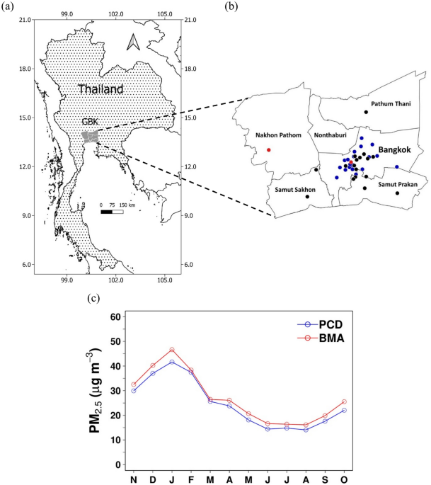
Hourly PM2.5 data was obtained for 17 monitoring stations in GBK monitored by the Pollution Control Department (PCD), and 20 monitoring stations in Bangkok monitored by the Bangkok Metropolitan Administration (BMA) (Fig. 1a, b). The study spans from November 2017 to October 2022, referred to as the 2018–2022 seasonal year. Satellite-derived Level 3 hourly AOD at 500 nm (referred to as AODmerged) was used as a proxy for atmospheric aerosols, sourced from the Japan Weather Agency’s Himawari-8 satellite30,31. This daytime data (08–17 Local Time) was downloaded from the Japan Aerospace Exploration Agency’s P-Tree System on the Himawari Monitor website (https://www.eorc.jaxa.jp/ptree/index.html) and is available at a spatial resolution of 0.05° × 0.05°. To evaluate the accuracy of AHI AOD, Level-3 sub-hourly ground-based AOD data at 500 nm for two AERONET (AErosol RObotic NETwork)32 stations in GBK (one each in Nakhon Pathom (NP) and Bangkok (BK) provinces respectively) were downloaded from https://aeronet.gsfc.nasa.gov (Fig. 1a, b). Reanalysis products from the 5th generation of the European Centre for Medium-Range Weather Forecasts (ECMWF), namely ERA5_LAND at a spatial resolution of 0.1° × 0.1° and ERA5 at a spatial resolution of 0.25° × 0.25° were selected for meteorological data. Given a better spatial resolution, ERA5_LAND was opted as the main reanalysis product which provides data for dew point temperature (DTEMP), global radiation (GR), air temperature (TEMP), u-component of wind (UWIND), and v-component of wind (VWIND). This was supplemented with mean sea level pressure (MSLP), planetary boundary layer height (PBLH), and cloud cover (CC) data from ERA5 (Table S2 in Supplementary Information). Relative humidity (RH) was calculated using DTEMP and TEMP as input using the humidity package in R33. All the meteorological data were obtained from the Climate Data Store (CDS; https://cds.climate.copernicus.eu). To account for the biomass burning in the region, daily active fires product (MCD14ML Collection 6.1) at 1 km resolution from MODIS sensors onboard the terra and aqua satellites were obtained (https://firms.modaps.eosdis.nasa.gov/download)34. As a proxy for vegetation cover, the Normalized Difference Vegetation Index (NDVI) from MODIS sensors of the terra (https://lpdaac.usgs.gov/products/mod13a1v061/)35 and aqua (https://lpdaac.usgs.gov/products/mod13a1v061/)35 satellites each produced at 16-day intervals at 500 m spatial resolution was used. Elevation data (HGT) was acquired from the Global Multi-Resolution Terrain Elevation Data 2010 from the United States Geological Survey at a spatial resolution of 7.5 arc seconds (~ 250 m). (https://topotools.cr.usgs.gov/gmted_viewer/viewer.htm). The population density (PD) data was obtained from the WorldPop database available at a spatial resolution of 30 arc seconds (~ 1 km) (https://www.worldpop.org/).

(a) Thailand and Greater Bangkok (GBK), (b) PM2.5 monitoring stations (PCD in Black and BMA in Blue) and AERONET stations (Red) in GBK, (c) Monthly variation of PM2.5 over averaged over PCD stations and BMA stations. In (c) the axis labels (N, D, J, F, M, …..S, O) denote the months of the year from November to October.
Data pre-processing
All gridded datasets were reprojected and regridded to a regular latitude/longitude grid of 0.05° × 0.05° to make them consistent with the grid size of AHI AOD. Next, the bilinear interpolation method was used to extract the values for different predictor variables for the location of PM2.5 monitoring stations. For forest fires, total FHS counts in 5 × 5 cells around the location of interest were used. For yearly datasets of PD and HGT, the same value was used for all the hours of the year. Sub-hourly to the hourly conversion of AERONET AOD was done and AHI AOD was computed as the average AOD within a spatial box that encompassed a 5 × 5 grid cells configuration, each measuring 0.05° × 0.05° and centered around AERONET monitoring sites. AHI AOD was evaluated against AERONET AOD using four statistical metrics. The mathematical description of these statistical metrics and results of satellite AOD evaluation are given in Section S2 and Table S3 in Supplementary Information. PM2.5 levels are relatively lower in the wet season during May–October and are not much of a concern but PM2.5 levels intensify in the dry season (Fig. 1c). Hence only dry season was considered for this study. The dry season has relatively less missing AOD but was still high enough to disrupt the continuous satellite-based air quality monitoring. Hence, AOD imputation was done using machine learning as used in previous studies too36,37 and discussed in Section S2 in Supplementary Materials.
Machine learning model development
A total of 13 predictor variables namely AOD, TEMP, RH, GR, UWIND, VWIND, CC, MSLP, PBLH, NDVI, FHS, HGT, and PD were used for PM2.5 estimation with six ML models. The selection of these predictor variables was based on their established relevance in influencing PM2.5 concentrations and usage in its prediction in previous studies9,10,11,12,13,14,15,16,17,18,19,20,21,22,23,27,28. AOD serves as a key proxy for surface PM2.5, capturing atmospheric aerosol loadings. Meteorological variables, including TEMP, RH, GR, UWIND, VWIND, CC, MSLP, and PBLH play a crucial role in PM2.5 formation, dispersion, and removal38. TEMP affects atmospheric stability and secondary aerosol formation while CC affects photochemical reactions and wet deposition processes. MSLP is linked to synoptic-scale weather patterns, governing air mass movements and pollutant accumulation or dispersion. GR is a key driver of photochemical reactions, influencing the formation of secondary aerosols, which contribute to PM2.5 mass. PBLH affects vertical mixing, relative humidity influences particle hygroscopic growth, and wind components determine pollutant transport38. Additionally, land surface and human activity indicators such as NDVI, FHS, HGT, and PD contribute to PM2.5 variations by representing vegetation cover, biomass burning events, air stagnation, and anthropogenic emissions, respectively. These variables collectively capture both natural and anthropogenic factors affecting PM2.5, ensuring a comprehensive representation of its variability. These ML models are random forest (RF)39, adaptive boosting or AdaBoost (ADB)40, gradient boosting (GB)41, extreme gradient boosting or XGboost (XGB)42, light gradient boosting machine or LightGBM (LGBM)43 and cat boosting or CatBoost (CB)44. These ML models were selected for PM2.5 estimation due to their widespread application in previous research highlighting their reliability and efficiency in predicting air quality10,11,12,13,14,15. These ML models can effectively capture complex, nonlinear relationships and interactions between variables. Ensemble approaches such as RF and boosting techniques enhance both accuracy and reliability, while advanced methods like XGB and LGBM are optimized for processing large datasets. Each ML model has distinct strengths and limitations that vary based on the dataset’s characteristics, such as sample size, number of features, etc. Hence, it is crucial to test and identify which delivers the best performance. A set of values for important hyperparameters for each ML model was selected based on previous studies11,12,13,14,15,26,27 and the author’s experience and different combinations of hyperparameters were tested for PM2.5 estimation. A set of values for important hyperparameters for each ML model was selected based on the author’s experience and different combinations of hyperparameters were tested for PM2.5 estimation. Nested cross-validation (CV) was used to optimize hyperparameters and evaluate model performance. In this method, a double-loop structure was employed in which the inner loop focuses on hyperparameter tuning, while the outer loop evaluates the model. During the inner loop, hyperparameters were optimized using Random Search with 5000 iterations and fivefold CV, where the data was split into five subsets, with four used for training and one for validation in each iteration. The best hyperparameters were selected based on their performance across these folds. In the outer loop, a tenfold CV was performed, where the data was divided into ten folds, with 90% used for training and 10% for testing in each iteration. This ensures that every data point is utilized for both training and testing while keeping the testing data independent of the tuning process. The average performance metric across the outer loop iterations provides an unbiased estimate of the model’s generalization ability, reducing the risk of overfitting and ensuring robust evaluation. The performances of various models were evaluated using the same statistical metrics applied during AOD evaluation. The final hyperparameters for each model were determined by tuning the models using the entire dataset for the dry season (as detailed in Table S2 of the Supplementary Information). The best-performing model was then utilized to estimate hourly PM2.5 levels for each grid cell.
Meteorological normalization for quantification of emissions and meteorological effects
Emission-related PM2.5 refers to the PM2.5_emis that can be quantified by decoupling the effect of the meteorology. Various methods have been developed to achieve this, each referred to by different terms. Traditionally, statistical models have been used for removing the effects of meteorology on PM10 or PM2.5. In this method, a statistical model (e.g., generalized linear model or generalized additive model) is developed for the relationship of the PM with meteorological, time-related (i.e. Julian day, day of the week, etc.), and other variables and then the PM concentration is adjusted for the effect of meteorology by extracting the effect of time-related variables plus intercept19. This is referred to as the meteorologically adjusted PM10 or PM2.5. Due to substantial development in the field of machine learning in the last two decades, it offers many ML models as alternatives to statistical models. Meteorological adjustment using ML was introduced by Grange et al. (2018)20 but referred it as meteorological normalization likely to distinguish this method from meteorological adjustment. In this method, first, an ML model is developed for PM2.5 prediction and then multiple predictions of PM2.5 for a specific time were done with randomly selected meteorological variables and then the predicted PM2.5 was averaged to obtain a normalized PM2.5 value. The number of predictions for each hour can be any large number. In this study, we resample meteorological variables for each hour 1000 times following Grange et al.20 and then took the average of these predictions as represented below:
$${PM}_{2.5\_emis}= \frac{1}{1000} \times \sum\limits_{i=1}^{1000}{PM}_{2.5, i (prd)}$$
(1)
Here, PM2.5_emis is the meteorologically normalized PM2.5 or emission-related PM2.5, while PM2.5, i, (prd) is the model predicted PM2.5 for the ith set of predictor variables. The best-identified ML model was used for meteorological normalization to estimate emission-related PM2.5. The meteorology-related PM2.5 (PM2.5_met) was calculated as the difference between predicted PM2.5 and emission-related PM2.5 as given below:
$${PM}_{2.5\_met}= {PM}_{2.5\_prd}- {PM}_{2.5\_emis}$$
(2)
Our approach builds on Grange et al. (2018)20 with modifications. We used the LightGBM model instead of the Random Forest model applied in their study and focused on PM2.5 rather than PM10. Additionally, while Grange et al. (2018)20 analyzed point observation data, we extended the approach to gridded PM2.5 data.
Spatiotemporal analysis of original and emission-related PM2.5
Spatial distribution of PM2.5 and PM2.5_met by hour of the day and month of the year were investigated. The trend in daily PM2.5 for each grid cell was computed using Theil-Sen Regression which computes the slopes and intercepts all possible combinations of subsample points and takes the median value which tends to give a more accurate confidence interval when assumptions on normality and homoscedasticity are not fulfilled by the datasets45. The significant trend of PM2.5 was estimated using the Mann–Kendall test. Theil–Sen trend analysis and the Mann–Kendall test were done using the trend package in R46. The stability analysis was done by calculating the coefficient of variation (COV). It is a statistical measure to calculate the relative variation in the dataset as the ratio of the standard deviation and mean of PM2.5 for each grid cell hence also called relative standard deviation. The persistence in PM2.5 was characterized by calculating the Hurst exponent (HE). The Hurst exponent (HE) is a statistical measure used to characterize the long-term memory or persistence in a time series. Here, the rescaled range (R/S) analysis was used to estimate the HE which was proposed by Hurst (1951)47 and later refined by Mandelbrot and Wallis (1969)48. The mathematical description for the HE is given by Jiang et al. (2015)49. The values for the HE range from 0 to 1 and are divided into three categories. HE < 0.5 indicates a time series with short-term memory and tends to return to its mean or exhibit anti-persistent behavior. HE = 0.5 suggests a purely random or uncorrelated time series. HE > 0.5 suggests a time series with long-term memory or persistent behavior. The pracma library in R50 was used for the estimation of HE.
SHAP analysis for PM2.5
The relative importance of different predictor variables on PM2.5 was investigated using the SHapley Additive exPlanation (SHAP) method, a concept derived from the field of cooperative game theory. SHAP analysis was used to understand the factors affecting PM2.5 because it provides a robust and interpretable framework for explaining the outputs of complex ML models24. It is widely validated in various studies, ensuring reliability and applicability across datasets 23,24,25,26,27. Furthermore, SHAP offers intuitive visualizations, making it easier to communicate findings and provide actionable insights for policymakers and researchers addressing PM2.5 pollution. When combined with ML models, this approach forms the basis of explainable ML. In explainable ML, predictions are first made using the ML model, and then each prediction is interpreted by attributing it to different predictor variables through the calculation of Shapley values. These values provide insights into the influence of each predictor variable on the model’s output by evaluating all possible combinations of variables and determining the average marginal contribution of each one. A positive Shapley value indicates that the variable has a positive effect on PM2.5 levels, while a negative value signifies a negative impact. Mathematically, the Shapley value is expressed as:
$${\varnothing }_{j}\left(val\right)=\sum_{S\subseteq \left\{{x}_{1}, {x}_{2}\dots \dots {x}_{p}\right\}\backslash {x}_{j}}\frac{\left|S\right|!\left(p-\left|S\right|-1\right)!}{p!}\left(val(S\cup \left\{{x}_{j}\right\})-val\left(S\right)\right)$$
(3)
Here, S represents a subset of the features used by the model, while x denotes the vector of feature values for the instance that is being explained. Additionally, p is the total number of features in the model. val (S) is the model’s prediction using only the features in subset S while \(val(S\cup \left\{{x}_{j}\right\}\) is the model’s prediction using the features in S along with the feature \({x}_{i}\). The SHAP values decompose the model prediction \(f\left(x\right)\) for instance x as the sum of the base value and the contributions of all features:
$$f\left(x\right)={\varnothing }_{0}+\sum_{i=1}^{p}{\varnothing }_{i}\left(x\right)$$
(4)
Here, \({\varnothing }_{0}\) is the base value, typically the expected value of the model’s output across all instances and \({\varnothing }_{i}\left(x\right)\) is the contribution of a feature \({x}_{i}\) to the prediction.
The base value \({\varnothing }_{0}\) is calculated as:
$${\varnothing }_{0}=E\left[f\left(x\right)\right]=\frac{1}{N}\sum_{i=1}^{N}f\left({x}^{\left(i\right)}\right)$$
(5)
Here, N is the number of training instances and \({x}^{\left(i\right)}\) is the i-th instance in the dataset. In this study also, we first predicted PM2.5 using the LGBM model and then calculated the Shapley values for each prediction instance. To identify the relative importance of different predictor variables, their mean absolute Shapley values were calculated. A Shapley value greater than 2 was set to identify key influencing factors for PM2.5. To comprehend the directional correlation between PM2.5 and the main influencing predictor variables, as well as to visualize the distribution of Shapley values associated with these predictors, global feature importance plots were used. The relationship between PM2.5 and key influencing variables was investigated using dependence plots.
Results and discussion
Performance evaluation of machine learning models
The results of the performance evaluation of different ML models in predicting hourly and daily PM2.5 using a tenfold CV are shown in Table 1. All models demonstrated reasonably good performance in predicting PM2.5 with relatively better performance on a daily time scale for all evaluation metrics except MBE. LGBM exhibited the best performance with the highest ρ at 0.9, zero MBE, lowest MAE at 5.5 μg m−3, and lowest RMSE at 8.7 μg m−3 for hourly PM2.5. The corresponding values for daily PM2.5 prediction are 0.95, − 0.01 μg m−3, 3.3 μg m−3, and 4.9 μg m−3. The values for ρ, MBE, MAE, and RMSE for different ML models ranged from 0.83 μg m−3 to 0.89 μg m–3, zero to − 0.63 μg m–3, 5.5 μg m−3 to 7.5 μg m–3, and 8.7 μg m−3 to 10.9 μg m–3 for hourly PM2.5 estimation. The corresponding values for daily PM2.5 are 0.88 to 0.96, − 0.01 μg m−3 to − 0.66 μg m–3, 3.3 μg m−3 to 5.9 μg m–3, and 4.9 μg m−3 to 8.2 μg m–3, respectively. LGBM outperformed RF, ADB, GB, XGB, and CB in PM2.5 estimation due to its combination of efficiency, scalability, and advanced algorithmic strategies tailored for complex datasets. Unlike RF, which builds multiple independent trees and averages their outputs, LGBM’s gradient-boosting approach sequentially refines predictions by focusing on reducing errors from previous iterations. This allows LGBM to capture intricate nonlinear relationships more effectively than RF. Additionally, LGBM’s leaf-wise tree growth strategy, which splits leaves with the highest information gain, results in deeper trees and better performance on datasets with complex patterns, such as PM2.5 variability influenced by multiple interdependent factors. Compared to ADB, which is robust but less adept at modeling complex relationships, LGBM’s ability to handle high-dimensional data and multiple feature interactions makes it more suitable for PM2.5 estimation. While GB and XGBoost also use gradient boosting, LGBM’s histogram-based algorithm reduces computation time and memory usage, making it significantly faster and more scalable for large datasets. It also includes advanced regularization techniques like L1/L2 and customizable loss functions, which help prevent overfitting which is a common challenge in air quality modeling. In comparison to CB, which excels in handling categorical data efficiently, LGBM benefits from its speed and optimized processing of numerical data, which often dominate PM2.5-related datasets. Furthermore, LGBM’s support for parallel and distributed computing makes it ideal for large-scale, computationally intensive tasks, such as estimating PM2.5 levels across multiple regions or long time periods. Aman et al.26 found that LGBM outperformed RF, ADB, GB, XGB, and CB, in visibility prediction at Bangkok Airport. Aman et al.27 compared different ML models for estimating PM2.5 in GBK and reported that ADB outperformed other ML models. Several global studies have compared machine learning models for PM2.5 estimation. Park et al.12 found that LGBM outperformed GB and XGB in Seoul, while Danesh Yazdi et al.51 and Shogrkhodaei et al.13 reported RF performed better than other models in London and Tehran, respectively. Chen et al.52 suggested a better performance by XGB as compared to RF and ADB in Central and Eastern China while Makhdoomi et al.53 found that GB outperformed RF, XGB, and LGBM in PM2.5 prediction over Mashhad city in Iran.
Spatiotemporal distribution in PM2.5 and PM2.5_met
The hourly spatial distribution of PM2.5 and PM2.5_met, are shown in Fig. 2. PM2.5 concentrations are higher in the morning (especially 08 LT–10 LT) and decrease gradually with time as the day proceeds. A positive value for PM2.5_met in the morning (especially 08 LT-11 LT) and negative values afterward over a larger region in GBK suggest that meteorology-related factors help in elevated PM2.5 level in the morning but help in improving air quality as the day proceeds. The observed patterns are closely related to changes in emissions and meteorological conditions over the daytime. In the morning hours, higher anthropogenic emissions are related to traffic congestion. Additionally, the thermal inversion layer is developed before sunrise leading to a decrease in boundary layer height leading to elevated PM2.5. As the day progresses post-sunrise, the thermal inversion layer dissipates, leading to an expansion of the atmospheric boundary layer’s height. This, in turn, facilitates the dispersion of air pollutants across a larger volume, resulting in a decrease in PM2.5 concentrations. The monthly spatial distribution of PM2.5 and PM2.5_met, are shown in Fig. 3. Higher PM2.5 during winter (especially during December and January) as compared to that during summer in March and April can be attributed to the synergetic effect of emissions from multiple sources and meteorological conditions6,54. Various studies on PM2.5 mapping in GBK have been done using statistical model55,56 or machine learning model27,29. Aman et al.27 estimated PM2.5 over GBK using Fengyun-4A AOD and other predictor variables using a stacked ensemble model developed by combining four ML models. Thongthammachart et al.29 developed a land use regression (LUR) model utilizing the LGBM model integrated with the Weather Research and Forecasting (WRF) model and the Community Multiscale Air Quality (CMAQ) model to predict daily ambient PM2.5 levels across Central Thailand. Peng-In et al.55 estimated PM2.5 over GBK using MODIS AOD and other predictor variables using linear regression model while Chalermpong et al.56 also used the LUR model for PM2.5 estimation over GBK. All these studies observed higher PM2.5 levels in winter compared to summer, consistent with the findings of this study. Similar patterns have also been reported in studies in other countries including studies by Dey et al.57 in India, Ma et al.9 in China, and Shogrkhodaei et al.13 in Tehran, Iran. A negative value for PM2.5_met over a larger area is found in November suggesting that meteorology helps in improving air quality. However, from December to February, positive values for PM2.5_met can be seen indicating a significant contribution by stagnant meteorological conditions during winter in air quality deterioration. During March and April as summer approaches, negative values for PM2.5_met over larger regions are again observed suggesting the role of meteorology in improving air quality.

Hourly spatial distribution of (a) PM2.5, (b) PM2.5_met.

Monthly spatial distribution of (a) PM2.5, (b) PM2.5_met.
Trend in PM2.5 and PM2.5_emis
The trend on daily PM2.5 and PM2.5_emis during dry, winter, and summer seasons and their significance (as reported by p-value) are shown in Fig. 4. During the dry season, 32.2% of total grids in GBK showed significant increasing trends (p-value < 0.05), 4.9% of total grids showed significant decreasing trends, and 62.9% of total grids showed no significant trends in PM2.5. Removal of the effect of meteorology on PM2.5 showed an increasing trend over 36% of the total area, a decreasing trend over 9.8%, and no trend over 54.1% of the total area. During winter, PM2.5_emis showed an increasing trend over only 15.6% area while PM2.5 showed an increasing trend over 67.8% of the total area. The percentage of areas showing a decreasing trend has also fallen sharply from 23.2% to 1.9%. A similar pattern was also found in the summer season when the percentage of areas showing an increasing trend increased from 18.7% to 34.6% while the percentage of areas showing a decreasing trend decreased from 12.6% to 6.5%. These results underscore the significant influence of meteorological factors in shaping PM2.5 trends. For instance, during winter, temperature inversions trap pollutants near the surface, preventing vertical mixing and causing a significant increase in PM2.5 levels, despite stable or reduced emissions. Similarly, low BLH during winter further restricts pollutant dispersion, intensifying air pollution. In contrast, higher BLH in the summer promotes better dispersion, but weak and inconsistent wind patterns can still lead to localized increases in PM2.5. The combined effects of these meteorological factors highlight that, although emission reductions have led to lower PM2.5 emissions in some areas, meteorological conditions significantly influence PM2.5 trends, limiting the effectiveness of mitigation efforts and emphasizing the need for targeted strategies that consider these factors. Various studies have quantified the emission-related PM2.5 using the ML model to assess the effectiveness of the PM2.5 mitigation strategies22,58,59. Qu et al.58 reported a significant decrease in emission-related PM2.5 after the removal of the effect of meteorology in the Beijing-Tianjin-Hebei (BTH) region between 2014 and 2019. Wang et al. (2022)22 reported a reduced rate of decline in PM2.5 levels and Xiao et al.59 observed a slower decreasing trend in PM2.5 over eastern China after applying meteorological normalization highlighting the need for stricter emission control policies.

(a) Trend and p-value in (a) PM2.5, (b) PM2.5_emis.
Stability and persistence of PM2.5
The variability characteristics of PM2.5 and PM2.5_emis in GBK during winter, summer, and dry seasons were studied using the COV as shown in Fig. 5. With regards to the spatial distribution, COV of PM2.5 is relatively higher over downtown Bangkok and regions adjacent to it as compared to areas in other provinces in GBK (Fig. 5a). The observed high COV in Bangkok can be attributed to the complex interplay of varying traffic patterns, and more pronounced localized meteorological effects such as urban heat island (UHI) effect, temperature inversions, and limited air circulation due to tall buildings. The UHI effect increases temperatures in Bangkok, enhancing atmospheric turbulence and altering wind patterns, leading to uneven pollutant dispersion across the city. While some areas experience dilution, others, especially those with limited ventilation, see pollutant accumulation. Additionally, higher temperatures accelerate secondary PM2.5 formation, contributing to spatial variability. Temperature inversions trap pollutants near the surface, preventing their dispersion and causing PM2.5 buildup in low-lying urban areas. These inversions lead to sharp fluctuations in pollution levels over time and across different parts of the city. The effect of meteorology on higher COV is evident from the spatial variation of COV of PM2.5_emis which is relatively lower in Bangkok and regions adjacent to it as compared to areas in other provinces further from Bangkok (Fig. 5b). The removal of meteorological effects on PM2.5 highlights the inherent emission patterns in the GBK. The local emission sources in Bangkok such as traffic, industries, and residential activities are more consistent as compared to emissions from agricultural residual burning in the nearby provinces. Hence PM2.5_emis has lower COV in Bangkok and nearby regions, highlighting the stable nature of pollution sources. In contrast, episodical emission from agricultural burning leads to higher COV even when meteorological effects are not considered. With regards to the temporal distribution, the COV of PM2.5 is higher in winter as compared to the summer (Fig. 5a). The winter season in GBK experiences low temperatures, sea breezes, and frequent arrival of cold surges from China which leads to frequent temperature inversions and stagnant weather conditions building up PM2.5 in the atmosphere causing haze episodes followed by clean days. In addition, the biomass burning in the local and nearby regions also causes short haze episodes7. On the contrary, the increase in temperature during the summer leads to dilution of PM2.5 causing lower and more stable concentration. COV of PM2.5_emis does not show any variation in different seasons and emissions patterns are relatively consistent over the dry season (Fig. 5b).

Coefficient of variation (COV) of (a) PM2.5 (b) PM2.5_emis.
The persistence of PM2.5 and PM2.5_emis in winter, summer, and dry seasons as analyzed with Hurst exponent is shown in Fig. 6. The minimum, maximum, and region-average values of the HEs are 0.62, 0.88, and 0.75 in the dry season, 0.62, 0.86, and 0.76 in winter, and 0.54, 0.89, and 0.72 in the summer season, respectively. For PM2.5_emis, these values are 0.6, 1.1, and 0.79 in the dry season, 0.58, 1.03, and 0.8 in winter, and 0.52, 1.09, and 0.73 in the summer season, respectively. The results suggest that GBK has weaker to stronger positive persistence in both PM2.5 and PM2.5_emis with slightly higher persistence of PM2.5_emis suggesting a persistence behavior by the emission sources when the effect of meteorology was removed. Both PM2.5 and PM2.5_emis showed higher persistence behavior in the winter season as compared to the summer season. During winter, meteorological conditions create an environment that favors the accumulation and prolonged presence of PM2.5 in the atmosphere. During winter, frequent temperature inversions trap PM2.5 near the surface, while a shallower planetary boundary layer limits vertical mixing, leading to higher concentrations. Weaker winds reduce horizontal dispersion, allowing pollutants to accumulate. Additionally, drier conditions result in less precipitation to remove PM2.5, unlike in summer when rainfall aids in pollutant washout. The persistence of PM2.5 in winter is also affected by increased seasonal emissions and limited pollutant dispersion. While industrial and traffic emissions remain relatively consistent year-round, biomass burning—particularly from agricultural residue burning and forest fires—intensifies during winter, releasing substantial particulate matter into the atmosphere. The spatial map suggests that persistence in PM2.5 is slightly lower in Bangkok compared to the region far away from Bangkok and this difference is even more pronounced in PM2.5_emis when the influence of change in weather conditions is removed. The lower persistence in Bangkok can be potentially attributed to the due to diverse and fluctuating emission sources and frequent regulatory interventions.

Hurst exponent (HE) for (a) PM2.5 (b) PM2.5_emis.
Drivers of PM2.5 pollution using SHAP analysis
The mean absolute SHAP value indicating the importance of different variables for the dry season is given in Fig. 7. The main variables affecting PM2.5, based on selected criteria of SHAP value > 2 are RH, PBLH, VWIND, TEMP, UWIND, GR, and AOD. The directional relationship and strength of influences of these variables on PM2.5 were investigated through partial dependence plots showing PM2.5 against SHAP values for each observation (Fig. 7). RH is the most important variable affecting PM2.5 with a mean absolute SHAP value of 5.29. The RHSHAP is mostly positive at very dry conditions (defined here as RH = 0–45%) and dry conditions (defined here as 45–60%), negative and positive both but with high-frequency of positive for low-humidity conditions (60–70%), mostly negative for mid-humidity condition (70–80%) and high-humidity condition (80–100%). These results suggest that at dry and low-humidity conditions RH has a positive relationship with PM2.5 exerting an accumulation effect which can be attributed to the persistence of suspended particles in dry air, limited particle growth, and lack of wet deposition. On the other hand, the high-humidity condition leads to a decrease in PM2.5 as at a high RH condition, air is saturated with water leading to the formation of clouds which lead to rain and reduce PM2.5 due to the wet scavenging effect60. PBLH is the second most important variable affecting PM2.5 having a mean SHAP value of 4.79. The PBLHSHAP is positive at lower PBLH (here defined as < 1 km) but negative at higher PBLH (here defined as > 1 km) suggesting higher PM2.5 when boundary layer height is shallow and vice-versa. When the PBLH is low, there is restricted vertical mixing of the air, causing pollutants like PM2.5 to be trapped in a smaller volume near the surface, which results in higher concentrations. Shallow PBLH combined with other favorable conditions such as low temperatures, and high RH can also accelerate the formation of secondary aerosols. When the PBLH is higher, vertical mixing of the air is more extensive, dispersing pollutants over a larger volume and reducing their concentration near the surface61,62. VWIND is the third important predictor variable with a mean SHAP value of 4.29. The inverted V shape shows that VWINDSHAP is mostly negative, and the negative values increase with an increase in the absolute value of VWIND i.e. both positive and negative. This suggests the decrease in PM2.5 concentration with an increase in the V component of wind. VWINDSHAP is positive at low absolute V wind component, suggesting an increase in PM2.5 concentration due to stagnant or less windy conditions. The next important predictor variable is temperature with a mean SHAP value of 3.68. The instance with positive TEMPSHAP is higher at lower temperatures and lower at higher temperatures suggesting the negative relationship of PM2.5 and temperature. Lower temperatures often correspond to a lower PBLH, trapping pollutants close to the ground and increasing PM2.5, whereas higher temperatures are associated with a higher PBLH, which enhances dispersion and reduces PM2.5 concentrations38. UWIND is the next important predictor variable with a mean SHAP value of 2.37. It showed a similar relationship with PM2.5 as VWIND. The negative value for UWINDSHAP increases with an increase in the absolute value of UWNID. However, the UWIND component is mostly negative. GR is the next important predictor variable with a mean SHAP value of 2.22. At lower GR, GRSHAP values are negative but are positive as GR increases. However, GRSHAP is less sensitive to GR as it increases. An increase in GR could potentially affect PM2.5 as it leads to an increase in temperature which can affect PM2.5 negatively due to an increase in PBLH leading to dilution of air pollutants. On the contrary, an increase in temperature could potentially increase secondary PM formation38. For AOD, the mean SHAP value is 2.03 with a negative AODSHAP value at lower AOD and a positive AODSHAP value at AOD > 0.4 (approx.). This suggests an obvious positive relationship between PM2.5 and AOD.

(a) Feature importance as measured by SHAP analysis (b) dependence plots of SHAP values for the key influencing variables.
Conclusions
This study used six machine learning (ML) models for surface PM2.5 estimation over Greater Bangkok (GBK) during the dry season of 2018–2022. The ML models are random forest (RF), adaptive boosting (ADB), gradient boosting (GB), extreme gradient boosting (XGB), light gradient boosting machine (LGBM), and cat boosting (CB). The predictor variables are aerosol optical depth (AOD), temperature (TEMP), relative humidity (RH), global radiation (GR), u component of wind (UWIND), v component of wind (VWIND), cloud cover (CC), mean sea level pressure (MSLP), planetary boundary height (PBLH), Normalized Difference Vegetation Index, fire hotspot counts (FHS), elevation (HGT), and population density (PD). LGBM exhibited the best performance for PM2.5 prediction, achieving the highest ρ (0.9 for hourly, 0.95 for daily), zero mean bias error (MBE), and the lowest MAE (5.5 μg m⁻3 hourly, 3.3 μg m⁻3 daily) and RMSE (8.7 μg m⁻3 hourly, 4.9 μg m⁻3 daily). The LGBM model was used for the estimation of PM2.5 over all grid cells in GBK. The spatial distribution of PM2.5 by hour suggests an elevated PM2.5 in the early morning between 08 and 10 LT which can be attributed to the hourly increased traffic emissions and the development of thermal inversion in the early morning. The breaking of the thermal inversion layer raises the boundary layer height, as the day proceeds leading to a decrease in PM2.5 concentrations. The spatial distribution of PM2.5_emis by hour suggests that meteorological factors contribute to higher PM2.5 levels in the morning but help in improving air quality as the day goes on. The monthly variation of PM2.5 suggests higher particulate pollution in the winter season as compared to the summer season, especially in Bangkok which experiences greater pollution levels than the surrounding provinces. Meteorology helped in improving air quality in November, March, and April months over a larger area while stagnant meteorological conditions in other months caused air quality deterioration. Trend analysis suggests that despite a reduction in emission-related PM2.5, PM2.5 levels increased over a larger region in GBK, indicating the limited effectiveness of mitigation measures in the region. A higher coefficient of variation (COV) of PM2.5 in winter can be potentially attributed to elevated PM2.5 with frequent changes in meteorological conditions that do not promote PM2.5 dilution. The spatial pattern of COV of PM2.5 and PM2.5_emis suggests that higher PM2.5 variability in Bangkok and nearby regions as compared to the other areas should be attributed to meteorology. The emission is more consistent over Bangkok as compared to the rural surroundings which experience episodical emissions from agricultural burning in the dry season. Both PM2.5 and PM2.5_emis show more persistent behavior in winter as compared to summer and this persistent behavior is less pronounced in Bangkok as compared to nearby regions. This could be potentially attributed to the fluctuating emission sources and regulatory interventions. SHAP analysis suggested RH, PBLH, VWIND, TEMP, UWIND, GR, and AOD as important variables affecting PM2.5. RH showed a positive relation with PM2.5 for very dry and dry conditions and a negative relation at higher humidity conditions due to wet scavenging. Low PBLH leads to higher PM2.5 concentrations due to limited air mixing, while higher PBLH decreases PM2.5 by dispersing pollutants. Wind speed has a negative relationship with PM2.5, as strong winds help reduce pollution. Temperature shows a negative relationship with PM2.5 as it increases at lower temperatures and vice versa. PM2.5 increases with an increase in global radiation initially but is less sensitive to radiation afterward. AOD positively correlates with PM2.5, indicating that higher aerosol levels correspond to increased PM2.5 concentrations. This study has certain limitations, as it relies on data-driven approaches using LightGBM and SHAP methods, which do not explicitly account for the underlying physical processes in the atmosphere. LightGBM, despite its strong predictive capability, remains sensitive to hyperparameter choices, requiring careful optimization to achieve the best performance. Even with optimized parameters, the model may have limited extrapolation capability, performing well within the range of training data but struggling to predict PM2.5 levels accurately under extreme conditions or in regions with significantly different air pollution dynamics. This limitation makes it less reliable for predicting unprecedented pollution events or adapting to areas with limited historical data. SHAP analysis does not inherently capture temporal dependencies, which are crucial for understanding long-term PM2.5 variations. This limitation may affect the model’s ability to distinguish between short-term fluctuations and persistent trends. Additionally, SHAP provides correlation-based attributions rather than causal relationships, meaning it cannot definitively determine whether a variable directly influences PM2.5 or is merely associated with another factor. Despite these limitations, SHAP remains a powerful and insightful tool for understanding the key drivers of PM2.5 variations. Its ability to quantify the contribution of different predictor variables for each instance enhances transparency and aids in better decision-making for air quality management. The following policy recommendations can be drawn from this study: (a) Policies should consider the seasonal dynamics of PM2.5, with enhanced efforts in winter when pollution levels are highest. (b) Despite reductions in emission-related PM2.5, overall PM2.5 levels have increased, highlighting the limited effectiveness of current mitigation measures. Policies should prioritize stricter enforcement of emission standards for traffic, industry, and agricultural burning, particularly during the dry and winter seasons when air quality deteriorates the most. (c) The impact of meteorological factors highlights the need to integrate its forecasting into air quality management, enabling early warnings and temporary measures like traffic restrictions or open burning bans. (d) Elevated PM2.5 levels and variability in Bangkok compared to surrounding regions emphasize the need for location-specific strategies in urban planning focusing on increasing green spaces, which can help reduce particulate matter. (e) Policymakers could allocate funding to harness the potential of satellite data and ML models for air quality predictions to support data-driven decisions. In the future, spatiotemporal mapping of PM2.5 can be enhanced by using advanced data-driven models, using additional predictor variables, and developing novel methods for very high-resolution PM2.5 mapping to capture PM2.5 variability at the hyperlocal scale. Developing a more homogeneous network of PM2.5 monitoring stations in GBK is also important to support urban-scale studies.
Data availability
The data used in the study are available upon request through the corresponding author, some of which may be subject to copyright.
References
Lelieveld, J., Evans, J., Fnais, M., Giannadaki, D. & Pozzer, A. The contribution of outdoor air pollution sources to premature mortality on a global scale. Nature 525, 367–371. https://doi.org/10.1038/nature15371 (2015).
Guo, Y. et al. The association between air pollution and mortality in Thailand. Sci. Rep. 4, 5509. https://doi.org/10.1038/srep05509 (2014).
Supasri, T., Gheewala, S. H., Macatangay, R., Chakpor, A. & Sedpho, S. Association between ambient air particulate matter and human health impacts in northern Thailand. Sci. Rep. 13, 12753. https://doi.org/10.1038/s41598-023-39930-9 (2023).
Pollution Control Department (PCD) (2024) Annual Report 2023, Pollution Control Department, Bangkok, Thailand (in Thai). https://www.pcd.go.th/wp-content/uploads/2024/06/pcdnew-2024-06-27_07-41-54_220443.pdf (accessed on 6th September 2024).
ChooChuay, C. et al. Impacts of PM2.5 sources on variations in particulate chemical compounds in ambient air of Bangkok, Thailand. Atmos. Pollut. Res. 11, 1657–1667. https://doi.org/10.1016/j.apr.2020.06.030 (2020).
Phairuang, W. et al. The influence of the open burning of agricultural biomass and forest fires in Thailand on the carbonaceous components in size-fractionated particles. Environ. Pollut. 247, 238–247. https://doi.org/10.1016/j.envpol.2019.01.001 (2019).
Aman, N. et al. A study of urban haze and its association with cold surge and sea breeze for Greater Bangkok. Int. J. Environ. Res. Public Health 20, 3482. https://doi.org/10.3390/ijerph20043482 (2023).
Kloog, I., Koutrakis, P., Coull, B. A., Lee, H. J. & Schwartz, J. Assessing temporally and spatially resolved PM2.5 exposures for epidemiological studies using satellite aerosol optical depth measurements. Atmos. Environ. 45, 6267–6275. https://doi.org/10.1016/j.atmosenv.2011.08.066 (2011).
Ma, Z., Hu, X., Huang, L., Bi, J. & Liu, Y. Estimating ground-level PM2.5 in China using satellite remote sensing. Environ. Sci. Technol. 48, 7436–7444. https://doi.org/10.1021/es5009399 (2014).
Xiao, F., Yang, M., Fan, H., Fan, G. & Al-qaness, M. A. A. An improved deep learning model for predicting daily PM2.5 concentration. Sci. Rep. 10, 20988. https://doi.org/10.1038/s41598-020-77757-w (2020).
Ma, J., Yu, Z., Qu, Y., Xu, J. & Cao, Y. Application of the XGBoost machine learning method in PM2.5 prediction: A Case Study of Shanghai. Aerosol. Air Qual. Res. 20, 128–138. https://doi.org/10.4209/aaqr.2019.08.0408 (2020).
Park, S. et al. Robust spatiotemporal estimation of PM concentrations using boosting-based ensemble models. Sustainability 13, 13782. https://doi.org/10.3390/su132413782 (2021).
Shogrkhodaei, S. Z., Razavi-Termeh, S. V. & Fathnia, A. Spatio-temporal modeling of PM2.5 risk mapping using three machine learning algorithms. Environ. Pollut. 289, 117859. https://doi.org/10.1016/j.envpol.2021.117859 (2021).
Tian, L. et al. The ground-level particulate matter concentration estimation based on the new generation of FengYun geostationary meteorological satellite. Remote Sens. 15(5), 1459. https://doi.org/10.3390/rs15051459 (2023).
Zhang, M. & Yuan, L. High-precision estimation of hourly PM2.5 concentration based on a grid scale of satellite-derived products. Atmos. Pollut. Res. 14, 101724. https://doi.org/10.1016/j.apr.2023.101724 (2023).
Kim, B. Y., Cha, J. W. & Lee, Y. H. Estimation of PM10 and PM2.5 using backscatter coefficient of ceilometer and machine learning. Aerosol. Air Qual. Res. 23, 230033. https://doi.org/10.4209/aaqr.230033 (2023).
Parde, A. N. et al. Estimation of surface particulate matter (PM2.5 and PM10) mass concentrations from ceilometer backscattered profiles. Aerosol. Air Qual. Res. 20, 1640–1650. https://doi.org/10.4209/aaqr.2019.08.0371 (2020).
Zhang, Q. et al. Drivers of improved PM2.5 air quality in China from 2013 to 2017. PNAS 116(49), 24463–24469. https://doi.org/10.1073/pnas.1907956116 (2019).
Barmpadimos, I., Hueglin, C., Keller, J., Henne, S. & Prévôt, A. S. H. Influence of meteorology on PM10 trends and variability in Switzerland from 1991 to 2008. Atmos. Chem. Phys. 11, 1813–1835. https://doi.org/10.5194/acp-11-1813-2011 (2011).
Grange, S. K., Carslaw, D. C., Lewis, A. C., Boleti, E. & Hueglin, C. Random forest meteorological normalisation models for Swiss PM10 trend analysis. Atmos. Chem. Phys. 18, 6223–6239. https://doi.org/10.5194/acp-18-6223-2018 (2018).
Grange, S. K. & Carslaw, D. C. Using meteorological normalisation to detect interventions in air quality time. Sci. Total Environ. 653, 578–588. https://doi.org/10.1016/j.scitotenv.2018.10.344 (2019).
Wang, M. et al. Slower than expected reduction in annual PM2.5 in Xi’an revealed by machine learning-based meteorological normalization. Sci. Total Environ. 841, 156740. https://doi.org/10.1016/j.scitotenv.2022.156740 (2022).
Hou, L. et al. Revealing drivers of haze pollution by explainable machine learning. Environ. Sci. Technol. Lett. 9, 112–119. https://doi.org/10.1021/acs.estlett.1c00865 (2022).
Lundberg, S. & Lee, S. I. A unified approach to interpreting model predictions. https://doi.org/10.48550/arXiv.1705.07874 (2017).
Wang, S., Ren, Y. & Xia, B. PM2.5 and O3 concentration estimation based on interpretable machine learning. Atmos. Pollut. Res. 14, 101866. https://doi.org/10.1016/j.apr.2023.101866 (2023).
Aman, N. et al. Estimating visibility and understanding factors influencing its variations at Bangkok airport using machine learning and a game theory-based approach. Environ. Sci. Pollut. Res. https://doi.org/10.1007/s11356-024-34548-4 (2024).
Aman, N. et al. Spatiotemporal estimation of hourly PM2.5 using AOD derived from geostationary satellite Fengyun-4A and machine learning models for Greater Bangkok. Air Qual. Atmos. Health 17, 1519–1534. https://doi.org/10.1007/s11869-024-01524-3 (2024).
Gupta, P. et al. Machine learning algorithm for estimating surface PM2.5 in Thailand. Aerosol. Air Qual. Res. 21, 210105. https://doi.org/10.4209/aaqr.210105 (2021).
Thongthammachart, T., Shimadera, H., Araki, S., Matsuo, T. & Kondo, A. Land use regression model established using light gradient boosting machine incorporating the WRF/CMAQ model for highly accurate spatiotemporal PM2.5 estimation in the central region of Thailand. Atmos. Environ. 297, 119595. https://doi.org/10.1016/j.atmosenv.2023.119595 (2023).
Bessho, K. et al. An introduction to Himawari–8/9—Japan’s new–generation geostationary meteorological satellites. J. Meteorol. Soc. Jpn. Ser. II(94), 151–183 (2016).
Xu, W., Wang, W. & Chen, B. Comparison of hourly aerosol retrievals from JAXA Himawari/AHI in version 3.0 and a simple customized method. Sci. Rep. 10, 20884. https://doi.org/10.1038/s41598-020-77948-5 (2020).
Holben, B. N. et al. AERONET-a federated instrument network and data achieve for aerosol characterization. Remote Sens. Environ. 66, 1–16. https://doi.org/10.1016/S0034-4257(98)00031-5 (1998).
Cai, J. An R package for calculating water vapor measures temperature and relative humidity. R package version 0.1.1. (2016). Available at: https://github.com/caijun/humidity. (accessed on 1st October 2023).
Giglio, L., Schroeder, W. & Justice, C. O. The collection 6 MODIS active fire detection algorithm and fire products. Remote Sens. Environ. 178, 31–41. https://doi.org/10.1016/j.rse.2016.02.054 (2016).
Didan, K. MODIS/Terra Vegetation Indices 16-Day L3 Global 500m SIN Grid V061. 2021, distributed by NASA EOSDIS Land Processes DAAC. https://doi.org/10.5067/MODIS/MOD13A1.061 (accessed on 10th October 2023).
Bi, J. et al. Impacts of snow and cloud covers on satellite-derived PM2.5 levels. Remote Sens. Environ. 221, 665–674. https://doi.org/10.1016/j.rse.2018.12.002 (2019).
Di, Q. et al. An ensemble-based model of PM2.5 concentration across the contiguous United States with high spatiotemporal resolution. Environ. Int. 130, 104909. https://doi.org/10.1016/j.envint.2019.104909 (2019).
Chen, Z. et al. Influence of meteorological conditions on PM2.5 concentrations across China: A review of methodology and mechanism. Environ. Int. 139, 105558. https://doi.org/10.1016/j.envint.2020.105558 (2020).
Breiman, L. Random forests. Mach. Learn. 45, 5–32. https://doi.org/10.1023/A:1010933404324 (2001).
Freund, Y. & Schapire, R. E. A short introduction to boosting. J. Jpn. Soc. Artif. Intell. 14, 771–780 (1999).
Friedman, J. H. Greedy function approximation: A gradient boosting machine. Ann. Stat. 29, 1189–1232. https://doi.org/10.1214/aos/1013203451 (2001).
Chen, T. & Guestrin, C. XGBoost: A scalable tree boosting system. In Proceedings of the 22nd ACM SIGKDD International Conference on Knowledge Discovery and Data Mining—KDD ’16, San Francisco, CA, USA, 785–794 (2016). https://doi.org/10.1145/2939672.2939785.
Ke, G. et al. LightGBM: A highly efficient gradient boosting decision tree. In Proceedings of the 31st Annual Conference on Neural Information Processing Systems (NIPS), Long Beach (2017).
Prokhorenkova, L., Gusev, G., Vorobev, A., Dorogush, A. V. & Gulin, A. CatBoost: Unbiased boosting with categorical features. NIPS’18: Proceedings of the 32nd International Conference on Neural Information Processing Systems, December 2018, 6639–6649.
Sen, P. K. Estimates of the regression coefficient based on kendall’s tau. J. Am. Stat. Assoc. 63, 1379–1389. https://doi.org/10.1080/01621459.1968.10480934 (1968).
Pohlert, T. trend: Non-Parametric trend tests and change-point detection. R package version 1.1.6. https://CRAN.R-project.org/package=trend. (accessed on 15th October 2023).
Hurst, H. E. Long-term storage capacity of reservoirs. Trans. Am. Soc. Civ. Eng. 116, 770–808. https://doi.org/10.1061/TACEAT.0006518 (1951).
Mandelbrot, B. B. & Wallis, J. R. Robustness of the rescaled range R/S in the measurement of noncyclic long run statistical dependence. Water Resour. Res. 5, 967–988. https://doi.org/10.1029/WR005i005p00967 (1969).
Jiang, W. et al. Spatio-temporal analysis of vegetation variation in the yellow river basin. Ecol. Indic. 51, 117–126. https://doi.org/10.1016/j.ecolind.2014.07.031 (2015).
Borchers, H. W. pracma: Practical numerical math functions. R package version 2.4.2. https://CRAN.R-project.org/package=pracma. (accessed on 1st October 2023).
Danesh Yazd, M. et al. Predicting fine particulate matter (PM25) in the Greater London Area: An ensemble approach using machine learning methods. Remote Sens. 12, 914. https://doi.org/10.3390/rs12060914 (2020).
Chen, J., Yin, J., Zang, L., Zhang, T. & Zhao, M. Stacking machine learning model for estimating hourly PM2.5 in China based on Himawari-8 aerosol optical depth data. Sci. Total Environ. 697, 134021. https://doi.org/10.1016/j.scitotenv.2019.134021 (2019).
Makhdoomi, A., Sarkhosh, M. & Ziaei, S. PM2.5 concentration prediction using machine learning algorithms: An approach to virtual monitoring stations. Sci. Rep. 15, 8076. https://doi.org/10.1038/s41598-025-92019-3 (2025).
Aman, N. et al. Visibility, aerosol optical depth, and low-visibility events in Bangkok during the dry season and associated local weather and synoptic patterns. Environ. Monit. Assess. 194, 322. https://doi.org/10.1007/s10661-022-09880-2 (2022).
Peng-In, B., Sanitluea, P., Monjatturat, P., Boonkerd, P. & Phosri, A. Estimating ground-level PM2.5 over Bangkok Metropolitan Region in Thailand using aerosol optical depth retrieved by MODIS. Air Qual. Atmos. Health 15, 2091–2102. https://doi.org/10.1007/s11869-022-01238-4 (2022).
Chalermpong, S., Thaithatkul, P., Anuchitchanchai, O. & Sanghatawatan, P. Land use regression modeling for fine particulate matters in Bangkok, Thailand, using time-variant predictors: Effects of seasonal factors, open biomass burning, and traffic-related factors. Atmos. Environ. 246, 118128. https://doi.org/10.1016/j.atmosenv.2020.118128 (2021).
Dey, S. et al. A satellite-based high-resolution (1-km) ambient PM2.5 database for India over two decades (2000–2019): Applications for air quality management. Remote Sens. 12(23), 3872. https://doi.org/10.3390/rs12233872 (2020).
Qu, L. et al. Evaluating the meteorological normalized PM2.5 trend (2014–2019) in the “2+26” region of China using an ensemble learning technique. Environ. Pollut. 266, 115346. https://doi.org/10.1016/j.envpol.2020.115346 (2020).
Xiao, Q. et al. Separating emission and meteorological contributions to long-term PM2.5 trends over eastern China during 2000–2018. Atmos. Chem. Phys. 21, 9475–9496 (2021).
Lou, C. et al. Relationships of relative humidity with PM2.5 and PM10 in the Yangtze River Delta, China. Environ. Monit. Assess. 189, 582. https://doi.org/10.1007/s10661-017-6281-z (2017).
Dupont, J. C. et al. Role of the boundary layer dynamics effects on an extreme air pollution event in Paris. Atmos. Environ. 141, 571–579. https://doi.org/10.1016/j.atmosenv.2016.06.061 (2016).
Stirnberg, R. et al. Meteorology-driven variability of air pollution (PM1) revealed with explainable machine learning. Atmos. Chem. Phys. 21, 3919–3948. https://doi.org/10.5194/acp-21-3919-2021 (2021).
Acknowledgements
The authors sincerely thank the Pollution Control Department (PCD) and Bangkok Metropolitan Administration (BMA) for providing the surface PM2.5 data. This research is supported by Ratchadapisek Somphot Fund for Postdoctoral Fellowship, Chulalongkorn University.
Funding
This study was supported by the Thai Health Promotion Foundation, under Center of Clean Air Solutions, grant number 68-E1-0083.
Ethics declarations
Competing interests
The authors declare no competing interests.
Additional information
Publisher’s note
Springer Nature remains neutral with regard to jurisdictional claims in published maps and institutional affiliations.
Supplementary Information
Rights and permissions
Open Access This article is licensed under a Creative Commons Attribution-NonCommercial-NoDerivatives 4.0 International License, which permits any non-commercial use, sharing, distribution and reproduction in any medium or format, as long as you give appropriate credit to the original author(s) and the source, provide a link to the Creative Commons licence, and indicate if you modified the licensed material. You do not have permission under this licence to share adapted material derived from this article or parts of it. The images or other third party material in this article are included in the article’s Creative Commons licence, unless indicated otherwise in a credit line to the material. If material is not included in the article’s Creative Commons licence and your intended use is not permitted by statutory regulation or exceeds the permitted use, you will need to obtain permission directly from the copyright holder. To view a copy of this licence, visit http://creativecommons.org/licenses/by-nc-nd/4.0/.
About this article

Cite this article
Aman, N., Panyametheekul, S., Pawarmart, I. et al. Machine learning-based quantification and separation of emissions and meteorological effects on PM2.5 in Greater Bangkok. Sci Rep 15, 14775 (2025). https://doi.org/10.1038/s41598-025-99094-6
Received:
Accepted:
Published:
DOI: https://doi.org/10.1038/s41598-025-99094-6