Comparative analysis of machine learning techniques for temperature and humidity prediction in photovoltaic environments

As a fundamental component of renewable energy production, Photovoltaic (PV) systems have been introduced as a sustainable and eco-friendly substitute for traditional fossil fuels¹. Solar PV systems capture the energy of the sun and convert it into electricity using semiconductor materials; they are essential in the move to more sustainable energy sources². Due to the growing demand of renewable energy; it is more important to improve the PV systems’ performance and efficiency^3,4,5,6. The energy production of these systems can be optimized not only to improve their economic feasibility, but also to help meet the goal of reducing carbon emissions and addressing climate change.

The external factors such as temperature and humidity greatly affect PV systems⁷. The electrical properties of PV cells may be influenced by temperature variations and this may affect their efficiency in converting sunlight to energy⁸. However, high temperatures can reduce the effectiveness of PV cells by increasing their internal resistance, and hence lower the energy production⁹. The performance of PV systems may be affected by humidity levels, leading to condensation, corrosion or deterioration of the materials the panels are made of¹⁰. Temperature and humidity play a significant role in the optimal operation and maintenance of PV systems¹¹, and therefore precise temperature and humidity forecasting is a necessity. Consequently, anticipating these environmental elements in advance will allow system configurations to be altered, maintenance tasks to be planned and precautionary measures applied to extend the life of the PV systems and ensure a constant energy output¹².

As the complexity and variability of climatic conditions have grown, there has been an increasing reliance on Machine Learning (ML) methods for predicting critical parameters affecting the efficiency of renewable energy systems, including PV systems¹³. This is where ML models are very well suited for this purpose because they can analyze huge datasets, detect patterns and establish relationships between input variables and outputs without requiring explicit programming¹⁴. In the field of renewable energy ML is important for precise and automated temperature and humidity forecasting. These are the factors that are necessary to maximize the efficiency of PV systems¹⁵. With the help of algorithms that can be adjusted to the ever changing environment, real time monitoring and forecasting is enabled by ML in PV systems¹⁶. The level of automation in these systems increases operating efficiency, reduces downtime, and results in more uniform energy output¹⁷. However, temperature and humidity forecasting in PV conditions is not trivial¹⁸. The energy production of PV systems has intricate and non-linear connections with temperature and humidity, which are environmental factors¹⁹. The accurate prediction of these correlations is difficult because of a number of factors, including geographic location, seasonal fluctuations, and local meteorological conditions²⁰. Moreover, temperature and humidity usually vary simultaneously, making the prediction modeling more complicated²¹. To provide accurate predictions, ML models need to include these ever changing interactions and at the same time reduce errors²². Such a high degree of accuracy can only be achieved with sophisticated algorithms that can deal with complex data, and many environmental factors. This highlights why it is important to pick the right ML methods for this particular use case¹⁴.

The reason for the comparative analysis of several ML techniques for temperature and humidity prediction is the imperative to improve the efficiency of PV systems. Different ML models may or may not be more or less effective in predicting environmental factors depending on the use case and the complexity of the data. Most previous research has been devoted to applying different models to different objectives of renewable energy forecast. However, the literature currently in publication lacks information on the best ML techniques to forecast temperature and humidity in PV environments. Therefore, to choose the most accurate and reliable models for this goal, a thorough review of various ML techniques is required. The accuracy and reliability of environmental forecasts is highly dependent on the choice of the ML model. Each algorithm has its own advantages and disadvantages, especially when it comes to their ability to deal with nonlinear relationships, feature interactions and unexpected data. Inaccurate predictions can result in ineffective management of solar power plants, which in turn will decrease energy output and increase stress on system components. As such, proper model selection is very important to improve prediction accuracy and to ensure long term efficiency and sustainability of PV systems. This research aims to determine the best models to improve decision making in PV system operations. This will enable increased energy output, timely maintenance, and more precise projections.

Motivated by missing a comprehensive comparison of all ML algorithms for temperature and humidity prediction in PV applications, this study provides a thorough comparison of eight common ML algorithms. In essence, the study aims at pursuing the most accurate and reliable models for predicting these essential climatic parameters that directly influence the PV systems performance and effectiveness. To this end explicitly, a wide range of ML techniques including Support Vector Regression (SVR), Linear Regression (LR), Ridge Regression (RR), Lasso Regression, Decision Tree (DT), Random Forest (RF), AdaBoost, Gradient Boosting (GB), and eXtreme Gradient Boosting (XGBoost) are examined. The rationale for selecting these models is identified on a broad range of approaches, simple LR methods and ensemble and boosting methods also. Among them, three primary measurement metrics were applied to compare the performance of each model, as follows: The Coefficient of Determination (R²), the Root Mean Squared Error (RMSE), and the Mean Absolute Error (MAE). These metrics offer a comprehensive evaluation of each model’s effectiveness in predicting temperature and humidity, allowing for a direct comparison of the models’ effectiveness in forecasting temperature and humidity in the specific context of PV environments through their error minimization capabilities and goodness of fit to the data.

This research contributes to the field of renewable energy by identifying the most effective ML models for predicting critical environmental parameters, including temperature and humidity, in PV systems. In this investigation, numerous ML algorithms, such as SVR, LR, Ridge, Lasso, DT, RF, AdaBoost, GB, and XGBoost, have been compared and contrasted to provide valuable insights into their respective advantages and disadvantages. The findings contribute to the expanding body of knowledge on the application of ML in PV systems and offer additional insight into the algorithms that are most effective for optimizing environmental forecasts. This research bridges the divide between the operational requirements of PV systems and the selection of ML models to enhance the overall performance and sustainability of PV systems. The practical implications of this research are extensive. Temperature and humidity are crucial for accurate forecasting, as they enable system administrators to optimize energy production by adjusting the settings in accordance with the anticipated conditions. Furthermore, the scheduling of maintenance duties is more effective due to the improved accuracy of environmental forecasts, which in turn delays the deterioration of the system and extends the lifespan of PV infrastructure. This research enhances the predictive capabilities of renewable energy systems and contributes to the overarching objectives of energy production optimization and the promotion of sustainable, data-driven solutions in the renewable energy sector.

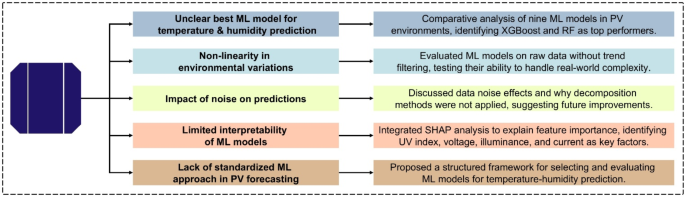
This study conducts a comparative analysis of multiple ML models to address critical challenges in temperature and humidity prediction for PV environments. The major challenges encountered in this domain and the corresponding contributions of this research are structured in Fig. 1. This research is remarkable for pointing out the most accurate ML models and evaluating their potential to fit non-linear environmental variability while investigating data noise impacts on prediction performance. In addition, Shapley Additive Explanations (SHAP) analysis can be used to increase the interpretability of the model, allowing for a better understanding of the main features driving predictions. To resolve the gap in standardized methodologies for PV forecasting, a structured ML evaluation framework is proposed to establish a systematic approach, which adapts with the ever-evolving ML domain.

Key challenges and contributions in ML-Based temperature and humidity prediction for PV environments.

The aim of this research is to predict system temperature and humidity in the PV environment, because these factors have a significant effect on efficiency and also the life span of a PV system. Unlike other studies involving the forecasting of weather-related variables, this study is highly applicable towards the realization of renewable energy generation forecasts of specific interest for the renewables industry, making it far more relevant to real-world concerns. Using nine different ML models, the study demonstrates a comparative methodology to examine the suitability of the different techniques for the purpose of PV optimization. Moreover, SHAP analysis integration improves model interpretability and provides essential insights into factors influencing PV performance within the environment. This case study’s finding enhance predictions for maintenance and monitoring in real-time for solar energy systems, leading to sustainable harvesting.

The study is structured systematically to ensure a clear progression from data acquisition to model evaluation. The Introduction provides background on PV systems, emphasizing the impact of environmental factors like temperature and humidity on their efficiency. It highlights the need for accurate forecasting using ML and justifies the comparative analysis of various ML models. The Methodology section details the research approach, beginning with Data Presentation, which describes the dataset, statistical summaries, and key environmental parameters. This is followed by an overview of ML Algorithms, covering model selection, training, and evaluation using MAE, RMSE, and R². The Results and Discussion section presents model comparisons, highlighting the superior performance of ensemble-based models like XGBoost and RF through visual analysis, including scatter plots, violin plots, and SHAP analysis for feature importance interpretation. The Future Work section explores advanced ML techniques, such as deep learning, optimization strategies, and real-time deployment for PV forecasting. Finally, the Conclusion summarizes key findings, emphasizing the advantage of ensemble models over traditional methods and suggesting further research to enhance real-time monitoring and predictive accuracy in PV systems.

Data presentation

In this section, the important variables in the dataset are shown visually and descriptive statistics are provided. It contains environmental and sensor based data including temperature, humidity, Ultraviolet (UV) index, voltage, current and illuminance.

In this study, the 5,000 sample dataset was divided into training and testing subsets for reliable assessment of the ML models. 80% of the dataset (four thousand samples) were held out for model training and allowed models to find patterns that existed under the surface information. The remaining 20% (1,000 samples) will be reserved for testing the models’ predicted ability on unobserved data and providing an independent evaluation. This split of the data makes the model not overfit the models on the dataset and also are able to generalize the models on the data which will be provided to the models at the end and beyond the training set.

The study’s primary variables—temperature, humidity, UV index, voltage, current, and illuminance—are summarized statistically in Table 1. With 5,000 observations for each variable in the dataset, a thorough foundation for comparing ML methods for temperature and humidity prediction in PV settings is provided.

With a standard deviation of 11.51 °C and a mean value of almost 15.06 °C, the temperature data reveals a broad range of observed temperatures. The measured temperatures range from 0.60 °C to 43.80 °C, representing the variety of environmental conditions that were recorded.

The range of humidity levels is from 10.10 to 65.20%, with a mean of 31.75% and a standard deviation of 12.01%. For the purpose of modelling meteorological conditions and how they affect PV systems, this humidity fluctuation is essential.

The UV index readings range from 0 to 8.41, with a mean of 1.39 and a standard deviation of 2.32. This suggests that the dataset encompasses intervals of both low and high UV exposure, which is crucial for comprehending how solar radiation affects humidity and temperature.

With averages of 6.14 V and 1.01 A, respectively, the voltage and current readings also show a great deal of variability, with the voltage peaking at 3.21 A and the current values reaching as high as 22.41 V. Analyzing the electrical performance of solar systems in various climatic situations requires an understanding of these variances.

With an approximate mean of 484.31 lx and a broad range from 46.45 lx to 1012.3 lx, the illumination clearly illustrates the breadth of different light conditions seen in the sample. Understanding how variations in light intensity impact temperature and humidity in PV settings depends on this variability.

All things considered, Table 1 offers a thorough synopsis of the dataset’s statistical characteristics, laying a strong basis for the next research and modelling projects. For the purpose of creating and assessing reliable ML models intended to precisely anticipate environmental conditions in solar systems, a wide range of data across all variables must be collected.

Histogram of temperature measurements: Frequency distribution of recorded temperatures in the dataset.

A range of temperature observations found in the dataset is shown in Fig. 2. Most of the temperatures recorded fall in the range 0 °C to 20 °C and thereby display a certain pattern in distribution. The most frequent reported temperatures are indicated by a prominent peak around 10 °C. This frequency declines incremental up to high temperature ranges such as from 30 °C to 40 °C, where fewer recording appeared. This means that the PV environment was predominantly characterized by lower and not very high temperatures. So, it shows not only how much heat is actually produced by this PV system but also what are particular humidity and temperature conditions in which this PV system was working, and it was working during the negative skewness of temperature distribution.

Histogram of humidity levels: Frequency distribution of recorded humidity values in the dataset.

Figure 3 displays the frequency distribution of the measured humidity values. Histogram showing a wide distribution of humidity, with the bulk of data lagging between 20% and 40%. The peak frequency occurs at 20% or so, which indicates that humidity levels in the PV environment were rather low. Above 40% it is an increasing scarce and above 60% is virtually non-existence. This distribution suggests that the PV system is regularly under dry conditions, which may be relevant in understanding how humidity influences the prediction of temperature in this type of environment.

Histogram of UV index values: Frequency distribution of recorded UV index measurements in the dataset.

The distribution of UV index values is shown in Fig. 4 with most of the recorded values between 0 and 1. A prominent spike is observed at the 0 line, indicating that a significant fraction of the observations is associated with very low or negligible levels of UV exposure. With just a few quantity of data obtained beyond a UV index of 2, the frequency drastically falls as the UV index increases. The low UV index readings suggest that the PV system operates in conditions when most of the time there is minimal direct sunlight or UV exposure. Accurate projection of the effect of UV exposure on the performance and temperature conditions of the system depends on this knowledge.

Histogram of voltage measurements: Frequency distribution of recorded voltage values in the dataset.

A bimodal pattern may be seen in the voltage measurement distribution, as seen in Fig. 5. There are a lot of readings that are concentrated around 0 V, which suggests that there are a lot of low or no voltage observations. This may be a sign of times when the PV system was not operating at all or was only getting very little electricity. The second peak appears at about 20 V, indicating that the system regularly functioned at this voltage level while it was in operation. The difference between these two peaks illustrates how the PV system operates, showing dramatic differences between periods of activity and inactivity.

Histogram of current measurements: Frequency distribution of recorded current values in the dataset.

Figure 6 shows a distribution of current measurements, which is also bimodal, similar to the voltage distribution. The maximum peak at 0 A indicated that the system often failed to detect current during periods of idleness or poor energy output. A second, lesser peak appears at 3 A, indicating that this level was primarily where current was created. The fact that the solar system often alternates between periods of inactivity and moderate energy output is further highlighted by this bimodal pattern.

Histogram of illuminance levels: Frequency distribution of recorded illuminance values in the dataset.

Similarly, the illuminance values presented in Fig. 7 also display bimodal distribution. The large clustering of observations around 0 lx suggests that the PV system faced conditions with little or no light for a substantial fraction of the time. This could refer to snapshots taken through the night or during other low light conditions. The second peak, detected at approximately 1000 lx, shows that under light stimulation the system frequently processed at relatively high illuminance levels. The distance between these two peaks shows both an incredible low and high illuminance by the system, with only small points of data in between.

Machine learning algorithms

ML Algorithms section provides a detailed examination of ML methods applied for the temperature and humidity prediction in solar systems. In this section, the model selection, training, and assessment procedures are examined, and the pros and cons of each approach are discussed. The analysis, incorporating factors such as complexity, feature handling, and interpretability, allows understanding of the trade-offs between model performance and usability. An analysis of ML techniques used in this study is also presented in this section, including a comparison framework to understand the efficacy of each model using Fig. 8; Table 2.

Through their capacity to manage substantial datasets and uncover intricate correlations among variables, ML models have been widely utilized in a range of environmental engineering fields. Other than predictive modeling monitoring in PV-based surroundings, ML techniques such as Artificial Neural Networks (ANN), Support Vector Machines (SVM), and ensemble-based of more than a few techniques are able to doing well in equivalent fields such as hydrological forecasting and water quality assessment. As an example, ANN and SVM were used successfully for river classification and to improve water quality monitoring in monsoonal environments, showing the adaptability of the algorithms for environmental modeling²³. Similarly, hybrid ML approaches combining ANN, Adaptive Neuro-Fuzzy Inference System (ANFIS), and Multiple Linear Regression (MLR) have been applied to predict heavy metal adsorption in water treatment, demonstrating their capability in handling nonlinear relationships and multi-variable dependencies²⁴. Furthermore, ensemble learning methods such as RF and optimized SVM models have been used for water quality index prediction, emphasizing the benefits of feature selection and model tuning for improving predictive accuracy²⁵. These studies reinforce the versatility of ML models in data-driven environmental predictions, supporting their applicability to temperature and humidity forecasting in PV systems.

The whole ML pipeline for predicting temperature and humidity in PV situations is depicted in Fig. 8. Importing the required libraries—such as pandas, numpy, and many ML and visualization libraries—is the first step in the process. The dataset is then entered into the software, where it is cleaned up by removing superfluous columns and using the median to manage missing values. This ensures that the data is ready for training models.

The flowchart then moves on to the feature engineering stage, when the target variables—heat and humidity—are separated from the pertinent characteristics, or independent variables. After that, the dataset is divided into training and testing sets so that the models may be trained on some data and their performance can be assessed on the remaining data.

Several ML models are initialised after feature engineering. These models include more sophisticated models like RF, GB, AdaBoost, and XGBoost in addition to more conventional models like DT and LR.

After that, the flowchart splits into two independent processes: one for predicting temperature and the other for predicting humidity. Predictions are made once the models in each branch have been trained on the appropriate data. Important measures, such as the R², RMSE, and MAE, are used to assess each model’s performance. To make it easier to compare the models, these assessment results are kept in DataFrames.

Lastly, bar charts that provide the performance metrics for the temperature and humidity forecasts are presented along with the data. When the assessment and visualization process is finished, the flowchart ends, clearly illustrating how well each model performs in forecasting temperature and humidity in PV situations.

ML workflow for temperature and humidity prediction in PV environments: A step-by-step representation of data preprocessing, feature selection, model training, evaluation, and visualization in the predictive modeling process.

A thorough comparison of ML techniques used in PV settings to forecast temperature and humidity is presented in Table 2. An understanding of the advantages and disadvantages of each of these algorithms is provided in Table 2, which lists the salient features of each algorithm.

The basic strategy used by every model is the kind of algorithm. For example, RR, Lasso Regression and LR are basic linear models that assume linear relationship between features and target variables¹³. These models are often the first to be considered when simplicity and interpretability are important. However, to deal with non-linear relationships and interactions between features, more advanced ensemble methods such as RF, AdaBoost, GB and XGBoost are designed²⁶. Consequently, these methods tend to achieve higher predictive accuracy, but at the cost of increased computational complexity and lower interpretability.

Each model is incredibly different in terms of complexity. Linear models are suitable in cases in which computational resources are scarce because they are simple to use and computationally economical¹³. However, models such as XGBoost and GB take more time and processing resource owing to their repeated training of many weak learners (typically DTs), and aggregation of predictions from them to improve the accuracy¹⁷.

Feature management varies in its sensitivity to data preparation when used with the models. For instance, SVR and linear models are sensitive to the size of the features, and need to be normalized or standardized for best performance¹⁹. However, ensemble techniques like RF and XGBoost are both capable of handling numerical and categorical data and are more impervious to feature scale changes¹⁷. Lasso Regression shines due to its ability to perform automated feature selection by efficiently reducing model complexity and dealing with multicollinearity issues¹³. This is achieved by shrinking the coefficients of less relevant features to zero.

Another crucial component to take into account is interpretability, particularly in applications where it’s crucial to comprehend the model’s decision-making procedure. Since the model coefficients clearly show how each feature and the target variable relate to one another, RR and LR are very interpretable¹³. Through their visual depiction, DT models also provide great interpretability, providing obvious insights into the decision-making process at each split in the tree. Nevertheless, interpretability declines with the use of more sophisticated models such as GB, AdaBoost, and XGBoost²⁶. Because it is challenging to determine how certain variables affect the final prediction due to the ensemble of weak learners, these models are sometimes referred to as “black box” models. In spite of this, they often perform better in terms of predicted accuracy than simpler models, particularly when working with complicated datasets.

An overall analysis of trade-offs between various algorithms, such as SVR, Lasso Regression, RR, LR, AdaBoost, GB, DT, RF, and XGBoost, based on complexity, feature handling, and interpretability is presented in Table 2^27,28,29. Simpler models can be more transparent, and require less processing power, but capture less intricate patterns in the data, whereas more complicated ensemble approaches capture more intricate patterns in the data at the expense of interpretability. Comparing these models is necessary to understand for what type of temperature and humidity prediction tasks each model is applicable, taking into account the accuracy versus interpretability trade off specific to the application.

This study did not utilize any decomposition strategy to address and reduce data noise prior to training the ML models. The main reason for this choice was to evaluate the inherent forecasting skills of various ML models in managing real-world environmental data without any preprocessing. High-frequency noise in temperature and humidity data can be filtered using decomposition techniques as Wavelet Transform, Empirical Mode Decomposition (EMD), or Seasonal-Trend Decomposition (STL), therefore adjusting the temperature and humidity data. Having said that, because they may find trends among several decision trees, some ensemble techniques like RF and XGBoost are naturally resilient to noise. On the other hand, simpler models like LR and SVR may have been more vulnerable to noise and they made more mistakes. Decomposition was not performed so some of this may have contributed to poor prediction, especially if the models can not handle noise. Future research will focus on the addition of decomposition methods as part of the ensemble model to understand their effect on the prediction accuracy and for generating more reliable predictions in the PV environment.

The study utilized nine different regression models from several libraries, including classical methods such as Decision Tree and LR, and ensemble methods such as RF, GB, and XGBoost, as summarized in Table 3. This study used their respective Python classes to access each model (for instance, “sklearn.tree.DecisionTreeRegressor” for the Decision Tree). By accommodating this suite of algorithms, a general comparison of predictive power and computational complexity over the PV setting can be performed.

As illustrated in Table 4, each regression model relies on a distinct set of key hyperparameters that regulate its training process and overall performance. Simpler models such as LR and RR have fewer settings (for example., “fit_intercept” or “alpha”), whereas more complex algorithms like XGBoost feature numerous adjustable parameters, including “learning_rate,” “max_depth,” and “subsample.” This variety highlights how tuning specific hyperparameters can significantly influence model behavior in terms of both predictive accuracy and computational complexity.

As highlighted in Table 5, each model was initially configured with default parameter settings to enable a fair, “out of the box” comparison. These defaults—which range from disabling maximum depth in Decision Trees (“max_depth = None”) to using moderate ensemble sizes (e.g., “n_estimators = 100” for both RF and GB)—generally offer balanced performance without extensive tuning. The accompanying remarks in Table 5 clarify how these defaults influence each algorithm’s behavior, underscoring, for example, the sensitivity of SVR to “C,” “epsilon,” and “gamma,” or the risk of overfitting in boosting-based models with large “n_estimators.”

Evaluation metrics

This study included three primary assessment measures to gauge the effectiveness of ML models in predicting temperature and humidity in PV settings. The metrics MAE, RMSE, and R² provide a thorough assessment of the accuracy and goodness-of-fit of the models^30,31,32,33. The MAE is a metric used to quantify the average size of mistakes in a given collection of predictions, regardless of their direction. The calculation determines the absolute discrepancy between the anticipated values and the actual values, providing a readily understandable measure of the accuracy of the forecast. Smaller MAE values imply superior model performance. Equation (1) is the formula for MAE. The RMSE is a measure that calculates the square root of the average of the squared discrepancies between projected values and actual values. RMSE is more sensitive to outliers compared to MAE since it penalizes greater mistakes more heavily by squaring the residuals. Similar to MAE, lower RMSE readings imply higher levels of prediction accuracy. RMSE is a valuable tool for comprehending the scale of prediction mistakes in the same units as the output variable. Equation (2) provides the formula for calculating the RMSE.

R² quantifies the amount of the variation in the dependent variable that can be accurately predicted by the independent variables. The metric offers a measure of how well the model fits the data, with values closer to 1 indicating a higher level of fit. A value of 1 for the R² shows that the model completely accounts for the variation in the data, while a value of 0 indicates that the model does not account for any of the variation. Equation (3) displays the formula R².

Recent studies in hydrology and climate forecasting have introduced alternative performance indices, such as the Combined Accuracy (CA) index, which integrates multiple error measures into a single metric to improve model assessment^34,35. The CA index has been applied in streamflow and hydroclimatic forecasting to enhance interpretability and provide a holistic evaluation of predictive performance. Future studies could explore the applicability of the CA index in ML-based temperature and humidity prediction models to determine whether it offers advantages over conventional accuracy measures.

Temperature prediction results

This subsection presents the performance evaluation of different ML models for temperature prediction using MAE, RMSE, and R² metrics. The results highlight the strengths and weaknesses of each model in capturing temperature variations in PV environments.

In this section, the study uses three important metrics—MAE, RMSE, and R²—to assess the effectiveness of several ML models for temperature prediction. Table 6 shows rounded to the closest thousandth the performance evaluation results for temperature prediction for every model across these criteria. Table 6 ranks the models from least to most efficient using the R² measure.

Figures 9, 10 and  11 exhibit a graphic depiction of the model performance concerning MAE, RMSE, and R² values. These graphs offer a simple reading of the errors and expected accuracy of the many models.

MAE comparison of ML models for temperature prediction.

SVR has the highest MAE, suggesting the largest average divergence from the actual temperature readings, as shown in Fig. 9, which shows the MAE for each model. XGBoost and RF, on the other hand, display significantly lower MAE values, indicating improved temperature forecast accuracy.

RMSE comparison of ML models for temperature prediction.

Figure 10 presents the RMSE values for each model, which reflect the square root of the average squared errors. Similar to the MAE, SVR demonstrates the highest RMSE, while XGBoost and RF again stand out with the lowest RMSE values, reinforcing their strong predictive performance.

R² comparison of ML models for temperature prediction.

The R² values quantifying the amount of variability as the model accounts for in the temperature data are presented in Fig. 11. The higher R² values represent a better fit of the model. RF and XGBoost have the highest R² value, while SVR lags behind with the least R² value, pointing out it fits worse than the other models.

This together with the data in Table 6 shows that XGBoost and RF are most efficient for temperature prediction because they have the lowest errors and the best fit to the data, whereas SVR is the worst across all metrics of evaluation.

In Fig. 12, this study presents scatter plots of predicted versus actual temperature values across nine different regression models: Fig. 12a SVR, Fig. 12b Lasso Regression, Fig. 12c RR, Fig. 12d LR, Fig. 12e AdaBoost, Fig. 12f GB, Fig. 12g Decision Tree, Fig. 12h RF, and Fig. 12i XGBoost. Points closer to the diagonal line indicate more accurate predictions, and each panel describes the correspondence between the model’s predictions and the actual temperatures. These subplots tell us at a glance which models do a better job of representing observed temperature trends.

Scatter plots of [redicted vs. actual temperature across various regression models: (a) SVR, (b) Lasso regression, (c) RR, (d) LR, (e) AdaBoost, (f) GB, (g) Decision tree, (h) RF, (i) XGBoost.

Figure 13 compares actual temperature readings with those expected by a range of regression models using violin graphs. Every “violin” shows the whole probability density of temperature values, therefore enabling the visualization of not only where expected values cluster but also the fluctuations of these values. One may get understanding of how precisely (and consistently) each model represents the observed temperature range by comparing the breadth and form of each model’s violin to the distribution of the real data.

Violin plot comparison of Actual vs. Predicted temperature across ML models. 

Humidity prediction results

This subsection analyzes the effectiveness of ML models in predicting humidity levels. The comparison based on MAE, RMSE, and R² values provides insights into each model’s ability to handle humidity fluctuations in PV environments.

Table 7 shows the ability of several ML models to predict humidity. The R² values are a crucial measure of model efficiency and the study provides a ranking of the models according to this metric in the Table 7. Lower R² values mean lower predictive ability, higher values mean better performance.

The results show that XGBoost performs the best with the lowest MAE (3.550), lowest RMSE (1.884) and highest R² (0.744). The results of these findings indicate that XGBoost is the most accurate and reliable model to predict humidity. RF is not far behind with similar performance, having a slightly higher MAE (3.583) and RMSE (1.893) but still quite robust R² (0.717). Clearly, these models are capable of successfully handling the complexity of the humidity prediction problem with a high degree of accuracy. However, SVR performs the worst with the highest MAE (6.780), the highest RMSE (2.604) and the lowest R² (0.253). It appears that SSVR has difficulty capturing the fundamental patterns in the data so that the prediction is less accurate. Furthermore, other models such as Lasso Regression, RR, and LR have moderate performance with R² between 0.457 and 0.468. However, when compared to XGBoost and RF, these models have much higher error metrics. AdaBoost shows a slight improvement with an R² value of 0.595, but remains below the most successful models in terms of both MAE and RMSE. The DT model has acceptable performance with MAE of 3.898 and RMSE of 1.974. However, with an R² of 0.649, its ability to explain variability in the humidity data is less than the more sophisticated ensemble approaches.

Figure 14 offers a graphic representation of the models’ MAE behavior. The SVR model clearly shows with the greatest MAE that it produces the largest average inaccuracy in humidity level prediction. Conversely, RF and XGBoost have the lowest MAE values, meaning their forecasts are more accurate than those of the other models.

MAE comparison of ML models for humidity prediction.

Figure 15 shows the RMSE values for every model, thereby clarifying the scale of the prediction errors. In keeping with the MAE findings, SVR shows the best RMSE—that is, equating to more prediction errors. Conversely, XGBoost and RF show improved performance once again owing to their reduced RMSE values, which results in less important error in their predictions.

RMSE comparison of ML models for humidity prediction.

Lastly, the models’ R² values are shown in Fig. 16. The most effective model for predicting humidity is XGBoost, which has the greatest R² value of 0.744. RF is next best, with an R² of 0.717. SVR, on the other hand, has the lowest R², highlighting even more how much less accurate it can predict than the other models.

R² comparison of ML models for humidity prediction.

Figures 14, 15 and 16; Table 7 show that SVR performs worse than the other models in every performance metric, while XGBoost and RF perform better at forecasting humidity and provide more accurate and consistent forecasts.

In Fig. 17, this study presents scatter plots of predicted versus actual humidity values for nine different regression models: Fig. 17a SVR, Fig. 17b Lasso Regression, Fig. 17c RR, Fig. 17d LR, Fig. 17e AdaBoost, Fig. 17f GB, Fig. 17g Decision Tree, Fig. 17h RF, and Fig. 17i XGBoost. The plots show how well each model reproduces the observed humidity, with lower deviations represented by closer points on the diagonal line. Two subplots create a visual representation and comparison to see how consistently each model is able to obtain the relationship between measured humidity and input features measured.

Scatter plots of predicted vs. actual humidity across various regression models: (a) SVR, (b) Lasso regression, (c) RR, (d) LR, (e) AdaBoost, (f) GB, (g) Decision tree, (h) RF, (i) XGBoost.

It also plots violins in Figure 18 showing the distribution of the actual humidity values against the predicted ones for different regression models. And each ‘violin’ holds a kernel density estimate from the data, showing where the values are more densely packed up — and how the values spread over the observed range. The final outputs of each model can give some comparison of the models about how accurately they replicate humidity conditions in reality, by comparing the shapes along with average lines of each model’s predicted distribution against the real humidity distribution.

Violin plot of actual vs. predicted humidity across various regression models.

SHAP analysis for feature importance in XGBoost

This study used SHAP analysis based on feature importance to help interpret predictions generated by the XGBoost model. The SHAP values show how much each feature contributed to the predicted temperature and humidity for each input, providing insight into how the model arrived at its predictions.

Figure 19 presents the SHAP summary plot for temperature prediction using XGBoost. The plot illustrates the effect of each input feature on the model’s output. Features with a higher SHAP value have a more significant impact on the prediction. In this case, UV index and voltage appear to be the most influential variables, as indicated by their wider distribution and strong effect on the temperature forecast. The color gradient represents the feature value, where red indicates higher values and blue represents lower values.

SHAP summary plot – XGBoost (temperature prediction).

Figure 20 illustrates the SHAP summary graphic for humidity prediction with XGBoost. The narrative emphasizes the comparative significance of many characteristics in forecasting humidity. Voltage and illuminance are the primary determinants, considerably influencing the model’s predictions. The distribution of SHAP values indicates that elevated voltage levels (red) significantly influence humidity estimates, whilst diminished illuminance values (blue) adversely affect the projected humidity levels.

SHAP summary plot – XGBoost (humidity prediction).

ANN:

Artificial neural network

ANFIS:

Adaptive neuro-fuzzy inference system

CA:

Combined accuracy

DT:

Decision tree

EMD:

Empirical mode decomposition

GB:

Gradient boosting

L1:

Lasso regularization

L2:

Ridge regularization

LIME:

Local interpretable model-agnostic explanations

LR:

Linear regression

MAE:

Mean absolute error

ML:

Machine learning

MLR:

Multiple linear regression

PV:

Photovoltaic

R² :

Coefficient of determination

RF:

Random forest

RMSE:

Root mean squared error

RR:

Ridge regression

SHAP:

Shapley additive explanations

STL:

Seasonal-trend decomposition

SVR:

Support vector regression

SVM:

Support vector machine

UV:

Ultraviolet

XGBoost:

EXtreme gradient boosting

Open access funding provided by The Science, Technology & Innovation Funding Authority (STDF) in cooperation with The Egyptian Knowledge Bank (EKB).

Funding provided by the Science, Technology and Innovation Funding Authority (STDF) in cooperation with the Egyptian Knowledge Bank (EKB).

Authors and Affiliations

1. Electrical Engineering Department, Faculty of Engineering, South Valley University, Qena, 83523, Egypt

   Montaser Abdelsattar & Ahmed AbdelMoety

2. Renewable Energy Science and Engineering Department, Faculty of Postgraduate Studies for Advanced Sciences (PSAS), Beni-Suef University, Beni-Suef, 62511, Egypt

   Ahmed Emad-Eldeen

Contributions

Montaser Abdelsattar, Ahmed AbdelMoety, and Ahmed Emad-Eldeen wrote the main manuscript text , prepared all the figures, and all authors reviewed the manuscript.

Corresponding author

Correspondence to Montaser Abdelsattar.

Competing interests

The authors declare no competing interests.

Publisher’s note

Springer Nature remains neutral with regard to jurisdictional claims in published maps and institutional affiliations.

Open Access This article is licensed under a Creative Commons Attribution 4.0 International License, which permits use, sharing, adaptation, distribution and reproduction in any medium or format, as long as you give appropriate credit to the original author(s) and the source, provide a link to the Creative Commons licence, and indicate if changes were made. The images or other third party material in this article are included in the article’s Creative Commons licence, unless indicated otherwise in a credit line to the material. If material is not included in the article’s Creative Commons licence and your intended use is not permitted by statutory regulation or exceeds the permitted use, you will need to obtain permission directly from the copyright holder. To view a copy of this licence, visit http://creativecommons.org/licenses/by/4.0/.

Reprints and permissions

References

Abdelsattar, M., Hamed, A. E., Elbaset, A. M., Kamel, A. A., Ebeed, M. & S. & Optimal integration of photovoltaic and shunt compensator considering irradiance and load changes. Comput. Electr. Eng. 97, 107658 (2022).
Oda, E. S. et al. Optimal allocation of a hybrid photovoltaic-based DG and DSTATCOM under the load and irradiance variability. Int. Trans. Electr. Energy Syst. 31, e13131 (2021).
Abdelsattar, M., AbdelMoety, A. & Ismeil, M. A. & Emad-Eldeen, A. Automated defect detection in solar cell images using deep learning algorithms. IEEE Access. (2025).
Abdelsattar, M., AbdelMoety, A. & Emad-Eldeen, A. Applying image processing and computer vision for damage detection in photovoltaic panels. Mansoura Eng. J. 50, 2 (2025).
Abdelsattar, M., AbdelMoety, A. & Emad-Eldeen, A. Machine learning-based prediction of illuminance and ultraviolet irradiance in photovoltaic systems. Int. J. Holist. Res., 1–14 (2024).
Abdelsattar, M., Ismeil, M. A., Azim, M. A. & AbdelMoety, A. & Emad-Eldeen, A. Assessing machine learning approaches for photovoltaic energy prediction in sustainable energy systems. IEEE Access. (2024).
Iqbal, S. et al. Impact and performance efficiency analysis of grid-tied solar photovoltaic system based on installation site environmental factors. Energy Environ. 34, 2343–2363 (2023).
Yang, Z. A comprehensive analysis of environmental factors affecting solar cells: dust accumulation, ambient temperature, and humidity. Appl. Comput. Eng. 23, 216–222 (2023).
Shiravi, A. H., Firoozzadeh, M. & Lotfi, M. Experimental study on the effects of air blowing and irradiance intensity on the performance of photovoltaic modules, using central composite design. Energy 238, 121633 (2022).
Makhija, A. S. & Bohra, S. S. Performance and degradation analysis for different solar photovoltaic technologies under hot and humid environment: a review. Progress Energy. 5, 042002 (2023).
Njok, A. & Kamgba, F. Monocrystalline photovoltaic panel response pattern to relative humidity and temperature under distinct wavelengths in Mangrove swamp environment in Calabar, cross river States, Nigeria. J. Appl. Sci. Environ. Manage. 27, 1825–1837 (2023).
Shaik, F., Lingala, S. S. & Veeraboina, P. Effect of various parameters on the performance of solar PV power plant: a review and the experimental study. Sustainable Energy Res. 10, 6 (2023).
Shakya, M. K., Pande, V. N., Kulkarni, R. S. & Kakade, S. 2023 International Conference on Digital Applications, Transformation & Economy (ICDATE). 240–244 (IEEE).
Kraemer, F. A., Asad, H. A., Bach, K. & Renner, B. C. Online machine learning for 1-day-ahead prediction of indoor photovoltaic energy. IEEE Access. 11, 38417–38425 (2023).
Sivakumar, S. et al. Machine learning approach on time series for PV-solar energy. Adv. Mater. Sci. Eng. 2022 6458377 (2022).
Kempelis, A., Narigina, M., Osadcijs, E., Patlins, A. & Romanovs, A. 2023 IEEE 10th Jubilee Workshop on Advances in Information, Electronic and Electrical Engineering (AIEEE). 1–6 (IEEE).
Raj, V., Dotse, S. Q., Sathyajith, M., Petra, M. & Yassin, H. Ensemble machine learning for predicting the power output from different solar photovoltaic systems. Energies 16, 671 (2023).
Karapanagiotis, C., Hicke, K. & Krebber, K. Optical Sensing and Detection VII. 213–219 (SPIE).
Tripathi, A. K., Sharma, N. K., Pavan, J. & Bojjagania, S. Output power prediction of solar photovoltaic panel using machine learning approach. Int. J. Electr. Electron. Res. 10, 779–783 (2022).
Pombo, D. V., Bindner, H. W., Spataru, S. V., Sørensen, P. E. & Bacher, P. Increasing the accuracy of hourly multi-output solar power forecast with physics-informed machine learning. Sensors 22, 749 (2022).
Howard, J. M. et al. Quantitative predictions of moisture-driven photoemission dynamics in metal halide perovskites via machine learning. J. Phys. Chem. Lett. 13, 2254–2263 (2022).
Mubarak, H. et al. 2022 IEEE global conference on computing, power and communication technologies (GlobConPT). 1–6 (IEEE).
Wong, Y. J. et al. Application of artificial intelligence methods for monsoonal river classification in Selangor river basin, Malaysia. Environ. Monit. Assess. 193, 438 (2021).
Wong, Y. J., Arumugasamy, S. K., Chung, C. H., Selvarajoo, A. & Sethu, V. Comparative study of artificial neural network (ANN), adaptive neuro-fuzzy inference system (ANFIS) and multiple linear regression (MLR) for modeling of Cu (II) adsorption from aqueous solution using Biochar derived from Rambutan (Nephelium lappaceum) Peel. Environ. Monit. Assess. 192, 439 (2020).
Sakaa, B. et al. Water quality index modeling using random forest and improved SMO algorithm for support vector machine in Saf-Saf river basin. Environ. Sci. Pollut. Res. 29, 48491–48508 (2022).
Mohamed, M., Mahmood, F. E., Abd, M. A., Chandra, A. & Singh, B. Dynamic forecasting of solar energy microgrid systems using feature engineering. IEEE Trans. Ind. Appl. 58, 7857–7869 (2022).
Xu, K., Xu, Y., Ye, Y. & Chen, W. Novel feature selection method for nonlinear support vector regression. Complexity 2022 4740173. (2022).
Wei, J. & He, X. Support vector regression model with variant tolerance. Meas. Control. 56, 1705–1719 (2023).
Roozbeh, M., Rouhi, A., Mohamed, N. A. & Jahadi, F. Generalized support vector regression and symmetry functional regression approaches to model the high-dimensional data. Symmetry 15, 1262 (2023).
Rights, J. D. & Sterba, S. K. R-squared measures for multilevel models with three or more levels. Multivar. Behav. Res. 58, 340–367 (2023).
Gao, J. R-Squared (R2)–How much variation is explained? Res. Methods Med. Health Sci. 5, 104–109 (2024).
Karatas, I. & Budak, A. Development and comparative of a new meta-ensemble machine learning model in predicting construction labor productivity. Eng. Constr. Architectural Manage. 31, 1123–1144 (2024).
Hodson, T. O. Root mean square error (RMSE) or mean absolute error (MAE): When to use them or not. Geosci. Model Dev. Disc. 2022 1–10. (2022).
Adnan, R. M. et al. Improved prediction of monthly streamflow in a mountainous region by Metaheuristic-Enhanced deep learning and machine learning models using hydroclimatic data. Theoret. Appl. Climatol. 155, 205–228 (2024).
Adnan, R. M. et al. Daily streamflow prediction using optimally pruned extreme learning machine. J. Hydrol. 577, 123981 (2019).