Identification of predictive subphenotypes for clinical outcomes using real world data and machine learning

Non-small cell lung cancer (NSCLC) is characterized by highly heterogeneous pathophysiology driven by differential biomarker expression in the tumor and surrounding microenvironment, immune response, and histology¹. NSCLC constitutes 80-85% of all lung cancers, with 75% diagnosed in advanced stages, resulting in a 5-year survival rate of 26.4%². Heterogeneity has also been observed across NSCLC patients in the incidence of underlying conditions, such as comorbidity burden and concomitant medication use. Despite tremendous progress in improving outcomes through immuno-oncology and other targeted approaches, the response remains heterogeneous.

To account for the complexity of diseases and individual variabilities, prediction medicine has been proposed with the goal of providing the right patient with the right treatment at the right time³. Data at different granularities, including omics, clinical, and environmental data, are required to comprehensively understand patients’ health conditions to achieve precision medicine. In addition to several national and international initiatives, including all-of-us⁴ and UK Biobank⁵, large-scale biomedical data have been collected over the years of scientific research and clinical practice^6,7,8, and machine learning methods have been developed and employed for extracting insights^9,10. These efforts have provided unprecedented resources and opportunities for transforming medicine.

However, there are challenges for developing individualized treatments arising from the heterogeneity of patient conditions, limited understanding of disease mechanisms, and imperfect capture of relevant patient biomarkers. As an intermediate step, stratified medicine¹¹ is an approach that identifies patient groups according to existing information, such as genetic markers^12,13,14, to ensure similar patient characteristics and response to treatment. Alternate approaches for deriving patient groups from data include unsupervised machine learning^15,16,17, although these methods cannot guarantee coherent outcomes within the groups.

In this work, we propose a general machine learning framework called Graph-Encoded Mixture Survival model (GEMS) to identify predictive subphenotypes from patient electronic health records (EHR). Each predictive subphenotype is a group of patients that shares similar baseline clinical characteristics and coherent within-group overall survival (OS), while ensuring distinct OS compared to other subphenotypes. GEMS was applied on a cohort of advanced NSCLC (aNSCLC) patients derived from a large US oncology EHR database. Our method yields superior quantitative performance in predicting individual treatment response compared to existing methods and identifies three predictive subphenotypes with distinct OS patterns.

Overview of the framework

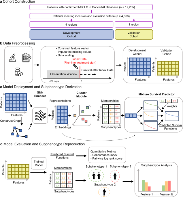
The overall workflow of our study is illustrated in Fig. 1. We constructed a cohort of aNSCLC patients treated with first-line (1 L) immune checkpoint inhibitor (ICI)-based therapies using a US oncology EHR database (ConcertAI Patient360™ NSCLC dataset; Jan 2015–Jan 2023)¹⁸. Each patient is represented by a 104-dimensional vector, with each dimension representing a variable extracted from their EHRs, including demographics, laboratory tests, vital signs, comorbidities, metastases, and medications (Fig. 1b, see Methods for more details).

a Construction of the full cohort and development and validation sub-cohorts. b Data preprocessing by extracting the feature vectors of patients from the EHR data. c Model deployment and derivation of subphenotypes in the development cohort. Our proposed model extracted efficient patient representations, clustered the patients into subphenotypes, and predicted survival distributions. d Model evaluation and reproduction of the subphenotypes on the validation cohort. Further analyses were conducted to interpret subphenotypes in both development and validation cohorts. ICI immune checkpoint inhibitor, NSCLC non-small cell lung cancer, GNN graph neural network. The microscope icon was made by iconnut, the health chart by Awicon, the medicine, syringe, and standing-up man by Freepik, and the neural network by pojok d, all obtained from Flaticon (www.flaticon.com) under appropriate licenses.

Our proposed model (GEMS) identifies patient groups as predictive subphenotypes associated with distinct real-world OS profiles (Fig. 1c). GEMS employs a Graph Neural Network (GNN) Encoder¹⁹ to effectively derive patient representations. Encoded patient representations are fed into a Clustering Module to cluster patients into predictive subphenotypes, which are used as base components in a Mixture Survival Predictor. The trained GEMS model was used to derive the predictive subphenotypes of ICI-treated aNSCLC patients (Fig. 1d).

Study cohort

Our study leveraged a retrospective, observational cohort sourced from deidentified data from the ConcertAI Patient360™ NSCLC dataset of histologically confirmed NSCLC patients (n = 17,265) between Jan 2015 and Jan 2023. There were 4666 patients included in this study, following the application of the inclusion/exclusion criteria and removing patients lacking valid OS records (Supplementary Fig. 1). This cohort had a mean (standard deviation) age of 68.69 ± 8.50 years, with 43.77% female (n = 2042) and 81.37% white (n = 3797). The median ([Q1, Q3]) OS was 314 [117, 684] days, observed among 71.09% of patients (n = 3317) that experienced death events.

We divided the cohort into model development and validation sub-cohorts based on US Census Bureau-defined geographic regions of the clinical institutions. Patients from the Northeast, South, and West regions were included in the sub-cohort (n = 3225, 69.12%) used for model development, while patients from the Midwest region (n = 1441, 30.88%) were used for independent validation. The development and validation sub-cohorts had similar demographics, including age (development, 68.68 ± 8.35; validation, 68.70 ± 8.80 years) and gender (43.54%; 44.27% female), while there was a higher proportion of white patients (validation, 88.75%; development, 78.08%) and patients from community institutions (93.62%; 84.99%) in the validation sub-cohort. Detailed summary statistics of the full cohort and the two sub-cohorts are provided in Table 1.

Quantitative performance

We compared the quantitative performance between GEMS and a set of baseline methods for predicting OS using the concordance index (c-index) as the performance metric²⁰ (see Methods for more details). We also reported the pairwise log-rank score²¹ for clustering methods. The baseline models included Cox proportional hazards regression (CPH)²², accelerated failure time (AFT)²³, survival support vector machine (SSVM)²⁴, gradient boosted decision trees (GBDT)²⁵, and neural survival clustering (NSC)²⁶. Additionally, we compared GEMS to unsupervised learning approaches, specifically K-means and hierarchical agglomerative clustering²⁷. For each method, we trained the model on the development cohort and evaluated the performance on the validation cohort.

The GEMS model achieved a mean c-index of 0.665 (95% confidence interval (CI): 0.662 – 0.667), compared to the best baseline c-index of 0.652 (95% CI: 0.650 – 0.655) achieved by GBDT (Table 2). The log-rank score obtained by GEMS was 69.17 (95% CI: 58.98 – 76.98), compared to the best baseline log-rank score of 56.23 (95% CI: 50.36 – 62.77) obtained by NSC. GEMS also outperformed unsupervised clustering baseline methods (K-means and hierarchical agglomerative clustering), highlighting the effectiveness of our framework in leveraging supervision from the data. Similarly, GEMS exhibited higher cross-validation c-index and pairwise log-rank scores compared to base methods in the development cohort (Supplementary Table 1).

We also evaluated the models for predicting time to progression or death from any cause (progression-free survival; PFS). To fit the GEMS model for PFS, we fine-tuned the survival prediction module to predict PFS, while keeping the GNN encoder and clustering modules fixed. The GEMS method outperformed baseline models in c-index and pairwise log-rank scores for predicting PFS (Supplementary Table 2).

We conducted a set of ablation studies to evaluate the impact of each module in the GEMS pipeline (Fig. 1c) and the training loss function on model performance. We compared the performance between GEMS and the following variants: (1) directly feeding the original patient feature vector to the cluster module; (2) replacing the GNN encoder with a multilayer perceptron (MLP) encoder; (3) eliminating clustering and significance loss; or (4) eliminating the significance loss from the loss function (see Methods for more details of the encoder and loss functions). Quantitative performance results of these ablation studies are shown in Supplementary Table 3. We observed that GEMS outperformed models without an encoder or using the MLP encoder, which suggests the value of considering the graph structure among the patient vectors. The GEMS model also outperformed models lacking clustering or significance loss terms.

We further characterized the effect of the GNN encoder on GEMS by visualizing patients and their GNN encoder-derived representations using uniform manifold approximation and projection²⁸ (UMAP). We leveraged the scDEED algorithm²⁹ to find the optimal hyperparameters for UMAP, as UMAP may not preserve global structure with inappropriate hyperparameters. Patients with different OS time are distinctly separated in UMAP space for the GNN encoder representations, compared to the original feature space where they are intermixed (Fig. 2).

a UMAP visualization on the original features. b UMAP visualization on the representations obtained by the GNN encoder. Individual data points represent patients and color scale represent OS times (log days). UMAP uniform manifold approximation and projection, GNN graph neural network. Source data are provided with this paper.

Predictive subphenotypes

We identified three predictive subphenotypes from the development sub-cohort. Demographics, smoking history, and OS statistics for each subphenotype are summarized in Table 3, with detailed baseline clinical characteristics in Supplementary Data 1. The OS Kaplan–Meier curves of the three subphenotypes are shown in Fig. 3a, and the incidence and co-incidence patterns on medications, metastasis, comorbidities, as well as clinical lab tests and vital signs with abnormal results across the 3 subphenotypes, are presented in Fig. 3b–d.

a Kaplan–Meier curves for overall survival (OS) for each subphenotype. The survival probabilities are shown by solid lines, and the shaded areas represent 95% confidence intervals around the curves. P-values are indicated in the figures; the numbers of samples to generate the curves are shown in the figures. b Group sunburst plot of administration rates of the medications across subphenotypes. The groups indexed by letters are determined based on the third level of anatomical therapeutic chemical (ATC3) class. c Chord diagrams of differences in metastasis (left), comorbidities (middle), and abnormal clinical feature classes (right) across subphenotypes. Ribbons indicate the normalized proportion of patients from a subphenotype to the corresponding feature class. d Graph of co-incidence patterns across subphenotypes. Each node within the network represents a specific feature, with its size proportional to the incidence within the particular subphenotype. The edge connecting a pair of nodes indicates the co-incidence of a corresponding feature pair, with the thickness proportional to the co-incidence rate; lines are displayed if the rate exceeds 5%. CHF congestive heart failure, FED fluid electrolyte disorders, CPD chronic pulmonary disease. Source data are provided with this paper.

Among the subphenotypes, Subphenotype 1 (n = 1335, 42%) had the highest proportion of females (55.50%) and the highest mean OS (688 days) (Table 3). Patients in this group exhibited the lowest medication administration rates for cough suppressants and expectorants (30.04%), beta-blocking agents (21.62%), general anesthetics (17.56%), angiotensin-converting enzyme (ACE) inhibitor combinations (44.58%), and antithrombotic agents (62.88%) (Fig. 3b). Subphenotype 1 patients also had lowest rates of bone (18.38%), adrenal gland (10.55%), and brain (18.75%) metastases (Fig. 3c, left). Finally, Subphenotype 1 exhibited the lowest proportion of patients with fluid electrolyte disorders (3.39%), congestive heart failure (4.13%), and diabetes (10.04%), and the lowest proportion of patients with abnormal renal clinical results (8.83%) (Fig. 3c, middle-right).

Subphenotype 2 (n = 420, 14%) had the lowest proportion of females (33.78%) among the three subphenotypes and mean OS of 454 days (Table 3). The hazard rate, or the speed of decrease in OS probability, for Subphenotype 2 was moderate in the first 500 days after 1 L initiation and subsequently peaked with disease progression (500-1000 days) (Fig. 3a). The proportion of patients with liver metastases (5.17%) was similar to Suphenotype 1 (4.67%) and lower than Subphenotype 2 (31.20%) (Fig. 3c, left). Patients in Subphenotype 2 exhibited moderate comorbidity burden and abnormal clinical results compared to the other subphenotypes, although proportion of patients with congestive heart failure was similar to Subphenotype 3 (8.67% and 8.73%, respectively).

Finally, Subphenotype 3 (n = 1420, 44%) was 35.21% female and had the lowest mean OS (321 days) among the subphenotypes. Patients in this subphenotype had the highest rates of medication administration (Fig. 3b), metastases to the liver (31.20%), bone (51.48%), adrenal gland (16.90%), and brain (25.77%), and baseline comorbidity burden for fluid electrolyte disorders (8.31%) and diabetes (15.14%) (Fig. 3c, left-middle). The proportion of patients with abnormal inflammatory (12.81%), hepatic (9.07%), and renal (21.43%) clinical results were highest for this subphenotype (Fig. 3c, right). Similarly, the co-incidence rates of metastases, comorbidities, and abnormal clinical tests in Subphenotype 3 were the highest amongst the subphenotypes (Fig. 3d).

Subphenotype reproducibility in the validation cohort

Subphenotypes were derived in the validation sub-cohort using the model trained from the development cohort. Demographics, smoking history, and OS statistics for each subphenotype are summarized in Table 4, with detailed baseline clinical characteristics in Supplementary Data 2.

Figure 4 describes the OS Kaplan–Meier curves, the association and co-incidence of baseline clinical characteristics for the validation cohort across subphenotypes. Subphenotype 1 (n = 586, 40.67%) had the highest mean OS (617 days) and the highest proportion of females (58.02%). Patients in Subphenotype 1 exhibited the lowest rates of metastasis across all sites, minimal comorbidity burdens for fluid electrolyte disorders and congestive heart failure, fewest abnormal values on renal tests, and lowest levels of medication administration. Subphenotype 2 (n = 224, 15.54%) had a lower proportion of females (40.62%) compared to Subphenotype 1 and moderate mean OS (473 days). Notably, its hazard rate was lowest within first 500 days of 1 L initiation and peaked with disease progression (500-1000 days), mirroring the trend observed in the development cohort. Subphenotype 2 had a low rate of liver metastasis (5.80%), while other characteristics, including metastasis sites, comorbidity burden, and abnormal clinical signs were moderate. Finally, Subphenotype 3 (n = 631, 43.79%) had the lowest mean OS (307 days) and the lowest proportion of females (32.81%). Patients in this subphenotype had the highest rates of metastases, comorbidity burden, and abnormal clinical results.

a Kaplan–Meier curves for overall survival (OS) for each subphenotype. The survival probabilities are shown by solid lines, and the shaded areas represent 95% confidence intervals around the curves. P-values are indicated in the figures; the numbers of samples to generate the curves are shown in the figures. b Group sunburst plot of administration rates of the medications across subphenotypes. The groups indexed by letters are determined based on the third level of anatomical therapeutic chemical (ATC3) class. c Chord diagrams of differences in metastasis (left), comorbidities (middle), and abnormal clinical feature classes (right) across subphenotypes. Ribbons indicate the normalized proportion of patients from a subphenotype to the corresponding feature class. d Graph of co-incidence patterns across subphenotypes. Each node within the network represents a specific feature, with its size proportional to the incidence within the particular subphenotype. The edge connecting a pair of nodes indicates the co-incidence of a corresponding feature pair, with the thickness proportional to the co-incidence rate; lines are displayed if the rate exceeds 5%. CHF congestive heart failure, FED fluid electrolyte disorders, CPD chronic pulmonary disease. Source data are provided with this paper.

In summary, our results in the validation sub-cohort exhibit similar trends to those derived in the development sub-cohort, indicating stability and reproducibility of the predicted subphenotypes. OS and baseline clinical and demographic characteristics are also similar between the sub-cohorts across subphenotypes.

Prediction of subphenotype membership using top features

To further understand the different characteristics across the subphenotypes, we tested the differences of each variable across the subphenotypes, ranked the variables based on the p-value (Supplementary Data 1), and selected the top 15 features on the development cohort for analysis. We compared the value distributions of these features across subphenotypes (Fig. 5a) and employed Shapley Additive Explanations (SHAP)³⁰ to quantify their impact on predicting subphenotype memberships (Fig. 5b).

a Distributions of the features across the subphenotypes. Bar charts indicate relative frequency for binary/ordinal features, while box plots are shown for continuous features. In all boxplots, the central bar in each box represents the median value of each respective category, the bounds of each box are the interquartile range (IQR), whiskers extend 1.5*IQR from each box, and the dots are the outliers. The numbers of samples to derive the statistics are shown in the figure. b Impact of the features on predicting the subphenotype membership, using Shapley Addictive Explanations (SHAP). Individual values of the features for each sample are colored according to their relative values, with the blue color representing lower values, and the red color representing higher values. The features are ranked based on mean absolute SHAP values. Positive SHAP values (> 0) indicate increased likelihood of subphenotype membership. ECOG Eastern Cooperative Oncology Group, NLR neutrophils-to-lymphocytes ratio, NMLR neutrophils and monocytes to lymphocytes ratio, WBC white blood cell. Source data are provided with this paper.

Of these 15 predictors, the Eastern Cooperative Oncology Group performance status (ECOG-PS) and total metastasis sites were consistently the top predictors for predicting subphenotype membership. Among the subphenotypes, Subphenotype 1 had the highest proportion of patients (90.2%) with ECOG-PS < 2 (90.2%) and total metastases <2 (87.7%), while Subphenotype 3 had highest proportion of patients with ECOG-PS ≥ 2 (44.0%) and total metastasis sites ≥ 2 (49.04%). Subphenotype 3 also exhibited a higher rate of liver metastasis (31.20%) than Subphenotypes 1 (4.67%) and 2 (5.17%). Subphenotype 2 had the highest proportion of patients with ECOG-PS = 1 (50.1%) and a single metastasis site (58.6%). Other top predictors included baseline laboratory test and vital signs. The neutrophil-to-lymphocyte ratio (NLR) and neutrophil and monocytes to lymphocytes ratio (NMLR) were key features distinguishing Subphenotype 2 from the other subphenotypes. Relative to Subphenotype 2, normal albumin levels, increased proportion of female patients, increased hematocrit, and reduced serum creatinine were key predictors of Subphenotype 1, while elevated heart rate, reduced oxygen saturation, increased alkaline phosphatase, and high white blood cell (WBC) counts were key predictors of Subphenotype 3.

In this study, we developed a general framework called GEMS to derive predictive subphenotypes that ensure the consistency of clinical characteristics and survival outcomes for patients in each subphenotype. We applied our framework to an EHR cohort of aNSCLC patients receiving 1 L ICI-based treatment and derived three distinct subphenotypes for predicting OS. These subphenotypes were consistent in their demographics, clinical characteristics, and OS between the geographically distinct development and validation sub-cohorts, indicating stability and reproducibility of our results.

Subphenotypes 1 and 3 comprised the majority of the patients in our study and corresponded to subpopulations with mild and severe baseline clinical characteristics, respectively. Subphenotype 1 (development, 42%; validation, 40.67%) had the highest proportion of female patients, lowest medication usage, lower rates of metastases and comorbidities, and fewer abnormal clinical test results compared to the other subphenotypes. Patients in this subphenotype were associated with the highest OS. By contrast, subphenotype 3 (44%; 43.79%) had more male patients with the highest rates of metastases and comorbidities and exhibited the largest proportion of patients with abnormal clinical test results. Patients in this subphenotype were associated with the lowest OS. Finally, Subphenotype 2 (14.40%; 15.54%) had the fewest patients amongst the three subphenotypes, with moderate baseline clinical characteristics and OS. Interestingly, the hazard rate in this subpopulation changed from moderate in the first 500 days following 1 L initiation to the highest amongst the subphenotypes with disease progression (500-1000 days). The identified subphenotypes were highly consistent across the development and validation cohorts, which were from different geographical regions.

SHAP analysis of top predictors of subphenotype membership was further used to understand differences between subphenotypes. These predictors have also been reported to be correlated with OS³¹. ECOG-PS and a total number of metastasis sites were key predictors of subphenotypes membership. This aligns with existing research indicating ECOG-PS as a prognostic factor for OS in aNSCLC^32,33. The presence of metastases, especially liver metastases, has also been linked to poor OS in aNSCLC patients compared to those without metastases^34,35. NLR and NMLR distinguished Subphenotype 2 from the other subphenotypes and have been reported as indicators of poor response to ICI therapy. Notably, the median ([Q1, Q3]) of NLR for Subphenotype 2 was 4.87 (3.57, 6.24), which encompasses previously reported clinically significant NLR thresholds of 3.98³⁶, 5³⁷, and 5.2³⁸. Compared to the other subphenotypes, patients in Subphenotype 2 were associated with poorer renal function, as evidenced by hypoalbuminuria and high serum creatinine, reduced red blood cell counts, and better cardiovascular function through normal heart rate and oxygen saturation. Oxygen saturation is an indicator of hypoxemia, which can reduce the effectiveness of ICI therapy³⁹. We also observed alkaline phosphatase as a key predictor for Subphenotype 3, which has been identified as a biomarker of ICI treatment response in NSCLC patients that are associated with liver and bone metastases⁴⁰. The interactions among these features suggest more complex pathophysiological mechanisms within the subphenotypes. For example, patients with mild to moderate renal insufficiency were observed to have lower hematocrit, while such association is even larger in men⁴¹. The above findings were consistent with the validation cohort (Supplementary Fig. 2). Similar results were obtained when the analysis was stratified by ECOG-PS and total metastases (Supplementary Fig. 3-8).

Our study has several strengths. First, the subphenotypes were derived based on the supervision of the OS outcome. Thus, distributions of OS were guaranteed to be coherent within each subphenotype and distinct across subphenotypes. Second, we divided the cohort into development and validation cohorts derived from distinct geographic regions in the United States. The consistent characteristics of the subphenotypes across cohorts validated the robustness of the derived subphenotypes. Third, the identified subphenotypes have distinct and clinically meaningful characteristics, which are supported by existing studies in aNSCLC. Finally, as the data format is generalizable as a feature vector and the training process is data-driven, our proposed framework can be applied to other disease analyses.

Our study also had some limitations. First, the subphenotypes derived from our method were determined based on the association between the features and the treatment response. Thus, the results did not lead to any causal conclusions. Identifying causality-based subphenotypes could be a valuable future research direction. Second, our study on aNSCLC was based on observational EHR data, which cannot explain the biological mechanisms behind aNSCLC. Third, we extracted information from structured and curated unstructured data without fully leveraging raw unstructured data such as physician notes, images, or reports. Fourth, comorbidities were determined using diagnosis codes, which may be miscoded and may not fully capture a patient’s actual comorbidity status. Furthermore, it is known that oncology EHR databases often suffer from under-reporting of concomitant medications, comorbidities, and tumor genomic profiling. Enhancing the current EHR database through tokenization and integration with claims databases could prove to be valuable. Sixth, due to lack of access to a non-ICI cohort, our study on aNSCLC was conducted exclusively within patients that received 1 L ICI. Consequently, the analysis is applicable only to patients receiving ICI therapy. Finally, our method used the most recent lab test and vital sign values prior to the index date as features. While incorporating longitudinal trends could enhance performance, most patients (58.6% on average) had ≤1 recorded result during the observation period in the ConcertAI data. Therefore, we leave the exploration of longitudinal information for future research using additional datasets with more comprehensive longitudinal information.

In conclusion, we developed a machine learning framework to identify the predictive subphenotypes for clinical outcomes. We evaluated the framework on an EHR-derived aNSCLC cohort with 1 L ICI treatment. Three reproducible subphenotypes were identified with distinct and clinically relevant characteristics. These findings offer valuable insights into the heterogeneity of aNSCLC patients. The results also demonstrated the effectiveness of our framework, suggesting its potential applicability to diverse disease contexts.

Ethics statement

The study was exempt from review by an institutional review board, and no waiver of authorization was required per US DHHS 45 CFR. Part 46 because it only used deidentified secondary data.

The ConcertAI EHR data repository

This study leveraged an observational, retrospective cohort derived from the ConcertAI Patient360™ NSCLC dataset, which is a U.S.-based, de-identified, patient-level dataset from the ConcertAI network that contains human abstracted variables from unstructured records in patients’ oncology EHR. The ConcertAI network comprises over 8 million unique patients from more than 900 oncology and hematology cancer clinics that leverage over 10 unique EHR environments. The dataset represents patients treated at both community and academic practices across all 50 U.S. states. The resulting abstracted data includes data elements including date and type of disease recurrence, histology, programmed cell death ligand-1 (PD-L1) testing information, tumor response, Eastern Cooperative Oncology Group performance status (ECOG-PS), and comorbidities.

Inclusion/exclusion criteria and outcomes

The study cohort was generated from the ConcertAI Patient360™ NSCLC dataset consisting of histologically confirmed NSCLC patients. The inclusion criteria for this study included confirmed diagnosis of locally advanced (stage IIIB/IIIC) or metastatic (Stage IV) NSCLC within 90 days prior to 1 L start, aged \(\ge\) 18 years at aNSCLC diagnosis date, and ICI-based monotherapy or combination therapies, with start of 1 L therapy (index date) between January 1, 2015 and January 30, 2023. Patients that were positive for aberrations to the epithelial growth factor receptor (EGFR), anaplastic lymphoma kinase (ALK), C-ros oncogene 1 (ROS1), Kirsten rat sarcoma virus (KRAS), or B-raf proto-oncogene (BRAF), received targeted therapies for those aberrations, or participated in a clinical trial after the aNSCLC diagnosis were excluded from the study.

Study setting

The observation period is stipulated as the 180 days antecedent to the index date. Overall survival (OS) is defined as time from the index date to all-cause death. Progression-free survival (PFS) is defined as time from the index date to the first real-world progression event or death from any cause. Real-world progression was derived from information abstracted by ConcertAI based on physician documentation of disease response, radiographic evidence, and pathology results^42,43,44. Censoring was performed at the earliest of the end of the study period or the patient’s last activity date in the EHR, ascertained from both structured and unstructured data (OS) or curated unstructured data only (PFS).

Different categories of variables were considered in our setting to predict clinical outcomes, including demographics, medical history, tumor characteristics, comorbidities, metastatic, concomitant medications, laboratory tests and vital signs. These variables were determined by clinical experts (Supplementary Data 3), with preprocessing according to the variable class:

Demographic variables

Demographic variables included age at the aNSCLC diagnosis date, gender, race, and practice type (community or academic).

Concomitant medications

The concomitant medications used during the observation period were collected. We categorized medications based on the third level of the anatomical therapeutic chemical (ATC3) classes⁴⁵. Each medication feature denotes the count of medications from its respective group used during the observation period.

Comorbidities and metastasis

Evaluation of comorbidities and metastasis was grounded on all documented International Classification of Diseases (ICD-9 and ICD-10) diagnoses within the observation period. The diagnoses were derived by rolling from ICD-9/10 codes to comorbidity classes provided in the HCUP/AHRQ Elixhauser comorbidity index⁴⁶. The comorbidity classes and their corresponding ICD-9/ICD-10 codes are presented in Supplementary Data 4.

Laboratory tests and vital signs

Laboratory tests and vital signs were identified from structured data using Logical Observations Identifier Names and Codes (LOINC) within the observation period. The LOINC codes of the lab tests are provided in Supplementary Data 5. For each test, the most recent value to the index date was utilized in the presence of multiple measurements.

Medical history

Smoking status (current or former) and baseline ECOG-PS were included, with most recent status preceding the index date utilized in the presence of multiple records within the observation period.

Biomarker status

Biomarker status variables were included. However, as the ConcertAI data is primarily from the community hospital setting rather than academic centers, full molecular testing panels are limited and may not be presented in reports. Thus, we retained biomarker variables that had at least 100 non-null samples (Supplementary Table 4).

Tumor characteristics

Tumor characteristics comprised tumor grade, histology, and PD-L1 expression level, determined through the comprehensive assessment of all valid PD-L1 percentage stain results obtained throughout the observation period.

Group stage

Ordinal encoding was employed for the feature of group stage, wherein Stage 0/I was designated as 0, Stage II as 1, Stage IIIA as 2, Stage IIIB/C as 3, and Stage IV as 4. As for other categorical variables, one-hot encoding was utilized, accompanied by the omission of one category from each variable to mitigate issues related to collinearity.

Considering data availability, we performed the following cleanup steps for feature selection:

• Removing features with high missing rates. Lab tests/vital signs with no recorded values for more than 80% patients during the observation period were excluded. Comorbidities, staging, and procedures are captured at lower frequencies in the ConcertAI database. To ensure retention of these feature classes, a more permissive missingness threshold (features with missingness > 95% were dropped) was used. As full molecular testing panels are limited and may not be presented in reports provided to the clinics; thus, the ConcertAI database has limited capture of full tumor genomic profiling. We retained biomarker variables that had at least 100 non-null samples to avoid preferential selection of variables, including genomic features.

• Removing highly correlated features. For each pair of features with correlation greater than 70%, we removed the feature with the higher missing rate. If both features had the same missing rate, the feature with the lower variance was removed. This process was repeated iteratively until no pairs of features with correlation greater than 70% remained.

After constructing and selecting the features, the missing values were imputed as: (1) zero for all comorbidities and metastases; (2) mode for categorical and binary features; and (3) mean for continuous features. The mode and mean values for imputation were calculated based on the development data and applied to both development and validation datasets. In order to eliminate the effects of value magnitude, all variables were scaled according to the z-score. More specifically, in the development cohort, z-score is calculated as \({x}^{{\prime} }=\frac{x-\mu }{\delta }\) where \(x\) is the value of a specific feature and \(\mu\) and \(\delta\) are the mean and standard deviation of the feature calculated over all samples on the development cohort, respectively. For the validation cohort, z-score is calculated using the same equation, with the mean and standard deviation of the development cohort.

The algorithm

The data we obtained was organized as follows: \({\left\{\left({{{\bf{x}}}}_{i},{\delta }_{i},{t}_{i}\right)\right\}}_{i=1}^{N}\) where \(i\) is the patient index and \(N\) is the total number of the patients. For the patient \(i\), \({{{\bf{x}}}}_{i}\) is the input feature vector, \({\delta }_{i}\) is the indicator variable with \({\delta }_{i}=1\) representing that an event occurred while \({\delta }_{i}=0\) indicating right-censoring, and \({t}_{i}\) is either the time of censoring (\({\delta }_{i}=0\)) or time of the event (\({\delta }_{i}=1\)).

Figure 1c illustrates the structure of the model. It consists of the following key components: (1) a Graph Neural Network (GNN) Encoder to learn effective patient representations, with a graph constructed with patients and their top 5 similar peers; (2) a Clustering Module that utilizes the patient representations from the GNN encoder to derive subphenotypes as graph partitions, resulting in cluster/subphenotype membership probabilities for each patient as output; (3) a Mixture Survival Predictor that incorporates the subphenotype membership probabilities as base components to build a mixture survival prediction model.

First, a graph was constructed with patients and their nearest neighbors. The vertices in the graph represent patients and the edges are connected between each patient and its top-5 nearest neighbors. The edges are weighted by the similarity between the pair of connected patients. We denote \({{\rm{dist}}}({{{\bf{x}}}}_{i},{{{\bf{x}}}}_{j})\) as the Euclidean distance between patients \({{{\bf{x}}}}_{i}\) and \({{{\bf{x}}}}_{j}\). The similarity between patients \({{{\bf{x}}}}_{i}\) and \({{{\bf{x}}}}_{j}\) is calculated as follows:

where \(\mu\) is an empirically tuned hyperparameter and \({\epsilon }_{i,j}\) is the normalized term calculated by the averaged distance of \({{{\bf{x}}}}_{i}\)(\({{{\bf{x}}}}_{j}\)) and their neighbors⁴⁷. The graph and feature matrix are input into a GNN encoder, which is implemented as a Graph Attention Network (GAT)⁴⁸, to derive patient representations. We denote the resulting representations for patient \(i\) output by the GNN encoder as \({{{\bf{z}}}}_{i}\).

The representation\({{{\bf{z}}}}_{i}\) is then fed into the clustering module to get the patient-specific cluster/subphenotype membership probabilities \({{{\bf{c}}}}_{i}=[{c}_{i}^{1},\ldots,{c}_{i}^{K}]\) as output, where \({c}_{i}^{k}\) indicates the probability of patient \(i\) belonging to the subphenotype \(k\) (\(0\le {c}_{i}^{1}\le 1,{\sum }_{k=1}^{K}{c}_{i}^{k}=1\)) and \(K\) is the number of subphenotypes. The clustering module is implemented with multilayer perceptron (MLP).

Finally, for each patient \(i\), the representation \({{{\bf{z}}}}_{i}\) and the cluster/subphenotype membership \({{{\bf{c}}}}_{i}\) are input into a survival predictor to get the predicted survival distributions for the patients. The survival predictor consists of \(K\) survival networks, where each survival network represents a hazard function \({g}^{k}\). \({g}^{k}({{{\bf{z}}}}_{i},t)\) is the estimated hazard rate at time \(t\) for patient \(i\) if patient \(i\) is in cluster/subphenotype \(k\). Then the patient’s hazard function is calculated as a weighted sum of these functions, with weights as the probability belonging to each cluster/subphenotype. That is, estimated hazard rate at time \(t\) for patient \(i\) is \({\sum }_{k=1}^{K}{c}_{i}^{k}{g}^{k}({{{\bf{z}}}}_{i},t)\).

The model was trained end-to-end to predict OS by minimizing a loss function composed of a survival prediction loss, which evaluates the accuracy of the survival prediction, a clustering loss aimed at ensuring coherence of patient representations within each subphenotype as well as differences across different subphenotypes, and a significance loss designed to ensure divergence of the averaged survival distributions across subphenotypes. The loss functions are calculated as follows:

Survival prediction loss

The survival prediction loss is defined as the log-likelihood of the survival time. We first denote the cumulative hazard function for the k cluster as \({\Lambda }^{k}({{{\bf{z}}}}_{i},t)={\int }_{0}^{t}{g}^{k}({{{\bf{z}}}}_{i},u){du}\). For the uncensored patients (\({\delta }_{i}=1\)), \({t}_{i}\) is the time of the event(death) and the likelihood of survival time being \({t}_{i}\) is: \({l}_{i}^{{{\rm{uncensor}}}}={\sum }_{k=1}^{K}{c}_{i}^{k}{g}^{k}\left({{{\bf{z}}}}_{i},{t}_{i}\right)\exp (-{\Lambda }^{k}({{{\bf{z}}}}_{i},{t}_{i}))\). For the censored patients, \({t}_{i}\) is the time of censoring (which means the event(death) has not happened until \({t}_{i}\)). The likelihood of surviving up to the censoring time is \({l}_{i}^{{{\rm{censor}}}}={\sum }_{k=1}^{K}{c}_{i}^{k}\exp (-{\Lambda }^{k}({{{\bf{z}}}}_{i},{t}_{i}))\). Combining the uncensored and censored patients, the overall survival prediction loss is as follows:

Clustering loss

We denote \({{\bf{C}}}\) as the whole membership matrix, whose \(i\)-th row is \({{{\bf{c}}}}_{i}\). We also denote \({{\bf{S}}}\) as the matrix of the weights of the edges. The clustering loss is defined as follows:

where \(m\) is the number of the edges in the patient graph.

Significance loss

For any pair of \({k}_{1}\) and \({k}_{2}\) (\({0\le k}_{1},{k}_{2}\le K,{k}_{1}\ne {k}_{2}\)), we use the log-likelihood ratio to quantify the significant difference between them⁴⁹. In particular, we first switch the predicted probabilities of clusters \({k}_{1}\) and \({k}_{2}\) for each \({{{\bf{c}}}}_{i}\), resulting in a membership distribution \({\widetilde{{{\bf{c}}}}}_{i}\)(\({\widetilde{c}}_{i}^{{k}_{1}}={c}_{i}^{{k}_{2}},{\widetilde{c}}_{i}^{{k}_{2}}={c}_{i}^{{k}_{1}}\) and \({\widetilde{c}}_{i}^{k}={c}_{i}^{k}\) for \(k\ne {k}_{1},{k}_{2}\)). Then we can calculate a log-likelihood loss by replacing \({{{\bf{c}}}}_{i}\) with \({\widetilde{{{\bf{c}}}}}_{i}\) in \({L}_{{{\rm{pred}}}}\), which is named \({L}_{{{\rm{switch}}}}({k}_{1},{k}_{2})\). If the discrepancy between the estimated survival functions in clusters \({k}_{1}\) and \({k}_{2}\) is larger, \({L}_{{{\rm{pred}}}}-{L}_{{{\rm{switch}}}}({k}_{1},{k}_{2})\) is larger. Thus, we define the significance loss as follows:

We conduct end-to-end training with a weighted loss function:

where \({\lambda }_{{{\rm{clus}}}}\) and \({\lambda }_{{{\rm{sign}}}}\) are hyper-parameters that could be determined empirically.

Evaluation

The model hyperparameters were first selected using 5-fold cross-validation on the training cohort. Since the number of the clusters is essential for subphenotype derivation, we tuned the number of the cluster and other model hyperparameters as follows:

We first set the number of clusters from 2 to 6. With each fixed number of clusters, we tuned the other hyperparameters by cross-validation and derived the phenotypes with the optimal hyperparameters. The ‘NbClust’ package was used to compute multiple metrics for clustering⁵⁰. The optimal number of clusters was determined by majority voting (Supplementary Table 5). After setting the number of clusters at three, we evaluated the performance of other hyperparameters, including a number of neighbors (Supplementary Table 6). The \({\lambda }_{{{\rm{clus}}}}\) and \({\lambda }_{{{\rm{sign}}}}\) determined by 5-fold cross-validation are 0.1 and 1.0, respectively.

With the determined hyperparameters and number of clusters, a model was trained on the full training cohort and evaluated on the independent validation cohort. To mimic the real-world scenario where the data from the development and validation cohorts could not be directly aggregated together to construct the graph, we trained and evaluated the model with our method under the inductive setting, where only patients in the development were used to construct the graph and train the model. During evaluation, the patients in the evaluation cohort were added to the graph to infer their predictions. To protect data privacy, the nearest neighbors were queried by locality-sensitive hashing (LSH)⁵¹.

To evaluate the performance on survival prediction, we utilized the concordance index (c-index), which assesses the effectiveness of the model in ranking patients according to their risk scores relative to the clinical outcomes of interest²⁰. The definition of concordance index is as follows:

where \({\eta }_{i}\) is the predicted risk for the patient \(i\).

We used the averaged pairwise log-rank score to quantify the clustering performance²¹. The log-rank score is a nonparametric statistic used to assess the similarity between two survival functions. It generates high values for curves that are highly unlikely to be similar. For \(K\) clusters, we calculate all possible pairwise comparisons and report the averaged results.

Baseline methods

We compared our proposed method with the following baselines:

The Cox proportional hazards regression (CPH) model is a semi-parametric model used to assess the influence of a specified set of features on the probability of an event happening⁵². In our study, we employed a penalized Cox regression approach, during which we fine-tuned the regularization parameter and selected a method to address tied event times^22,52.

The accelerated failure time (AFT) model is a parametric approach for survival prediction²³. In our analysis, we employed quantile-quantile (QQ) plots to assess the goodness of fit for our two outcomes and ultimately selected the log-logistic AFT model. This model assumes a linear relationship between recovery time and covariates. We further optimized the rate of false positives and the weights for penalization.

The Survival Support Vector Machine (SSVM) can effectively manage right-censored survival data by integrating ranking-based and regression-based loss functions²⁴. Its computational efficiency was enhanced through the utilization of kernel functions. We fine-tuned the weights for penalization, the mixing parameter between ranking and regression loss, and the choice of optimizers to optimize the model’s performance.

We also utilized Gradient Boosted Decision Trees (GBDT) in our study²⁵, using the Cox loss function for GBDT for the survival data. Learning rate, number of regression trees, maximum depth of the individual regression estimators, and the fraction of samples to be used for fitting the individual regression estimators were tuned.

The Neural Survival Clustering (NSC) is a deep learning state-of-the-art survival method that utilizes clustering for survival prediction²⁶. The survival distribution is represented with a mixture of positive and monotone neural networks, which represent the cumulative hazard functions for the clusters. We tuned hyper-parameters of the learning rate, number of hidden layers, and number of nodes in each hidden layer for this method.

The K-means and Hierarchical Agglomerative Clustering (HAC) are two types of unsupervised clustering methods. To evaluate performance for predicting survival, these methods were first applied to the baseline data to obtain cluster identity for each patient. Cluster identities were then used in the mixture survival predictor with the same model structure as in our framework to derive survival times, which were trained separately.

For all baseline methods, we followed the same procedure as with our proposed method to tune the hyperparameters by cross-validation.

Statistical analysis

We tested the statistical differences for each variable across subphenotypes by first identifying statistically significance (p < 0.05). Continuous variables were tested using one-way analysis of variance or the Kruskal–Wallis test for normal and non-normally distributed variables, respectively. Categorical variables were tested using the one-sided Fisher’s exact test. Post-hoc pairwise analysis between subphenotype pairs was performed for variables where overall p-value < 0.05. For each pair of subphenotypes, continuous variables were tested using Tukeyʼs honestly significant difference test or the pairwise Wilcoxon rank sum test for normal and non-normally distributed variables, respectively, and categorical variables were tested using the pairwise Fisherʼs test.

Subphenotype visualization

The incidence and co-incidence patterns on medications, metastasis, comorbidities, as well as clinical lab tests and vital signs with abnormal results across subphenotypes were visualized using the following plots.

Group sunburst plot

Group sunburst plots in Figs. 3b and 4b were generated to illustrate the administration rates of the medications during the observation period across subphenotypes. The groups indexed by letters are determined based on the third level of the anatomical therapeutic chemical (ATC3) class.

Chord diagram plot

Chord diagram plots in Figs. 3c and 4c were created to visualize the patterns of metastasis, comorbidities, and abnormal clinical tests (laboratory tests, vital signs) across subphenotypes.

• We assessed five metastasis sites: liver, bone, adrenal gland, brain, and pleura. Each ribbon in the chord diagram indicates the normalized proportion of patients within a subphenotype who had a specific metastasis site.

• We assessed four comorbidities: congestive heart failure (CHF), fluid electrolyte disorders (FED), diabetes, and chronic pulmonary disease (CPD). Each ribbon in the chord diagram indicates the normalized proportion of patients within a subphenotype who had a specific comorbidity.

• We grouped the lab tests and vital signs into the following categories: (1) Inflammatory markers: white blood cell (WBC) counts, albumin, lactate dehydrogenase, monocytes percent, basophils percent, eosinophils percent, albumin/globulin (A/G) ratio; (2) Hepatic markers: blood bilirubin total, aspartate aminotransferase (AST), alanine aminotransferase (ALT), alkaline phosphatase; (3) Cardiovascular markers: heart rate, systolic blood pressure, diastolic blood pressure, oxygen saturation; (4) Renal markers: serum creatinine, blood urea nitrogen, chloride, sodium. (5) Hematologic markers: serum plasma glucose, platelets, hematocrit.

Then we used the reference range to determine whether a lab/vital test is abnormal or not for each patient. Each ribbon in the chord diagram represents the normalized proportion of patients within a subphenotype who had at least one abnormal result in the above clinical group. The reference ranges and abnormality characteristics of the lab test and vital features are shown in Supplementary Table 7.

Group co-incidence graph

For each subphenotype, we drew a network to show the co-incidence relationships between the features (Figs. 3d and 4d). On the graph, each node corresponds to a variable (metastasis, medications, groups of lab tests, and vital signs), each edge corresponds to co-incidence, with thickness proportional to the co-incidence rate.

Reporting summary

Further information on research design is available in the Nature Portfolio Reporting Summary linked to this article.

Authors and Affiliations

1. Department of Population Health Sciences, Weill Cornell Medicine, Cornell University, New York, NY, USA

   Weishen Pan, Zhenxing Xu, Qiannan Zhang & Fei Wang

2. Regeneron Pharmaceuticals, Inc., Tarrytown, NY, USA

   Deep Hathi & Ying Li

Contributions

W.P., Y.L., and F.W. proposed the initial idea and designed the framework. W.P. and Q.Z. implemented the framework. W.P. analyzed the results. D.H. and Z.X. set up the data infrastructure and analytics environment and processed the ConcertAI data. W.P. and F.W. wrote the initial draft of the paper. F.W., Y.L., and D.H. made critical revisions. F.W. supervised the project. All authors have provided feedback and proofread the final version of the paper.

Corresponding author

Correspondence to Fei Wang.

Competing interests

D.H. is an employee and shareholder of Regeneron Pharmaceuticals, Inc. Y.L. is an employee and shareholder of Regeneron Pharmaceuticals, Inc. The remaining authors declare no competing interests.

Peer review information

Nature Communications thanks Xiao Luo and the other, anonymous, reviewer(s) for their contribution to the peer review of this work. A peer review file is available.

Open Access This article is licensed under a Creative Commons Attribution-NonCommercial-NoDerivatives 4.0 International License, which permits any non-commercial use, sharing, distribution and reproduction in any medium or format, as long as you give appropriate credit to the original author(s) and the source, provide a link to the Creative Commons licence, and indicate if you modified the licensed material. You do not have permission under this licence to share adapted material derived from this article or parts of it. The images or other third party material in this article are included in the article’s Creative Commons licence, unless indicated otherwise in a credit line to the material. If material is not included in the article’s Creative Commons licence and your intended use is not permitted by statutory regulation or exceeds the permitted use, you will need to obtain permission directly from the copyright holder. To view a copy of this licence, visit http://creativecommons.org/licenses/by-nc-nd/4.0/.

Reprints and permissions

References

Chen, Z., Fillmore, C. M., Hammerman, P. S., Kim, C. F. & Wong, K.-K. Non-small-cell lung cancers: a heterogeneous set of diseases. Nat. Rev. Cancer 14, 535–546 (2014).
Ganti, A. K., Klein, A. B., Cotarla, I., Seal, B. & Chou, E. Update of incidence, prevalence, survival, and initial treatment in patients with non-small cell lung cancer in the US. JAMA Oncol. 7, 1824–1832 (2021).
Collins, F. S. & Varmus, H. A new initiative on precision medicine. N. Engl. J. Med. 372, 793–795 (2015).
The ‘All of Us’ research program. New England Journal of (2019).
Palmer, L. J. UK Biobank: bank on it. Lancet 369, 1980–1982 (2007).
Gottesman, O. et al. The Electronic Medical Records and Genomics (eMERGE) Network: past, present, and future. Genet. Med. 15, 761–771 (2013).
Hripcsak, G. et al. Observational Health Data Sciences and Informatics (OHDSI): Opportunities for Observational Researchers. Stud. Health Technol. Inform. 216, 574–578 (2015).
Fleurence, R. L. et al. Launching PCORnet, a national patient-centered clinical research network. J. Am. Med. Inform. Assoc. 21, 578–582 (2014).
Jordan, M. I. & Mitchell, T. M. Machine learning: Trends, perspectives, and prospects. Science 349, 255–260 (2015).
LeCun, Y., Bengio, Y. & Hinton, G. Deep learning. Nature 521, 436–444 (2015).
Trusheim, M. R., Berndt, E. R. & Douglas, F. L. Stratified medicine: strategic and economic implications of combining drugs and clinical biomarkers. Nat. Rev. Drug Discov. 6, 287–293 (2007).
Hall, I. P. Stratified medicine: drugs meet genetics. Eur. Respir. Rev. 22, 53–57 (2013).
Matthews, P. M., Edison, P., Geraghty, O. C. & Johnson, M. R. The emerging agenda of stratified medicine in neurology. Nat. Rev. Neurol. 10, 15–26 (2014).
Mathai, S. K., Newton, C. A., Schwartz, D. A. & Garcia, C. K. Pulmonary fibrosis in the era of stratified medicine. Thorax 71, 1154–1160 (2016).
Fereshtehnejad, S.-M., Zeighami, Y., Dagher, A. & Postuma, R. B. Clinical criteria for subtyping Parkinson’s disease: biomarkers and longitudinal progression. Brain 140, 1959–1976 (2017).
Xu, Z. et al. Sepsis subphenotyping based on organ dysfunction trajectory. Crit. Care 26, 197 (2022).
Zhang, H. et al. Data-driven identification of post-acute SARS-CoV-2 infection subphenotypes. Nat. Med. 29, 226–235 (2023).
Products & Services. ConcertAI https://www.concertai.com/products/ (2020).
Zhou, J. et al. Graph neural networks: A review of methods and applications. AI Open 1, 57–81 (2020).
Harrell, F. E. Jr, Lee, K. L. & Mark, D. B. Multivariable prognostic models: issues in developing models, evaluating assumptions and adequacy, and measuring and reducing errors. Stat. Med. 15, 361–387 (1996).
Mantel, N. Evaluation of survival data and two new rank order statistics arising in its consideration. Cancer Chemother. Rep. 50, 163–170 (1966).
Stanford University. Department of Statistics, Stanford University. Division of Biostatistics & Efron, B. The Efficiency of Cox’s Likelihood Function for Censored Data, (1975).
Wei, L.-J. The accelerated failure time model: a useful alternative to the Cox regression model in survival analysis. Stat. Med. 11, 1871–1879 (1992).
Pölsterl, S., Navab, N. & Katouzian, A. Fast training of support vector machines for survival analysis. in Machine Learning and Knowledge Discovery in Databases: European Conference, ECML PKDD 2015, Porto, Portugal, September 7-11, 2015, Proceedings, Part II 15 243–259 (Springer, 2015).
Friedman, J. H. Stochastic gradient boosting. Comput. Stat. Data Anal. 38, 367–378 (2002).
Jeanselme, V., Tom, B. & Barrett, J. Neural Survival Clustering: Non-parametric mixture of neural networks for survival clustering. Proc. Mach. Learn Res 174, 92–102 (2022).
Jain, A. K., Murty, M. N. & Flynn, P. J. Data clustering: a review. ACM Comput. Surv. 31, 264–323 (1999).
McInnes, L., Healy, J., Saul, N. & Großberger, L. UMAP: Uniform Manifold Approximation and Projection. J. Open Source Softw. 3, 861 (2018).
Xia, L., Lee, C. & Li, J. J. Statistical method scDEED for detecting dubious 2D single-cell embeddings and optimizing t-SNE and UMAP hyperparameters. Nat. Commun. 15, 1753 (2024).
Lundberg, S. M. & Lee, S.-I. A unified approach to interpreting model predictions. Adv. Neural Inf. Process. Syst. 4765, 4774 (2017).
Li, Y. et al. Machine learning models for identifying predictors of clinical outcomes with first-line immune checkpoint inhibitor therapy in advanced non-small cell lung cancer. Sci. Rep. 12, 17670 (2022).
Gridelli, C. et al. Treatment of advanced non-small-cell lung cancer patients with ECOG performance status 2: results of an European Experts Panel. Ann. Oncol. 15, 419–426 (2004).
Dall’Olio, F. G. et al. ECOG performance status ≥2 as a prognostic factor in patients with advanced non small cell lung cancer treated with immune checkpoint inhibitors-A systematic review and meta-analysis of real world data. Lung Cancer 145, 95–104 (2020).
Tamura, T. et al. Specific organ metastases and survival in metastatic non-small-cell lung cancer. Mol. Clin. Oncol. 3, 217–221 (2015).
Ashour Badawy, A. et al. Site of metastases as prognostic factors in unselected population of stage iv non-small cell lung cancer. Asian Pac. J. Cancer Prev. 19, 1907–1910 (2018).
Murray, J. C. et al. Peripheral myeloid cells as prognostic markers in patients (pts) with non-small cell lung cancer (NSCLC) treated with cemiplimab: Pooled analysis of EMPOWER-Lung 1 and EMPOWER-Lung 3 phase 3 trials. J. Clin. Orthod. 41, 9028 (2023).
Ayers, K. L. et al. A composite biomarker of neutrophil-lymphocyte ratio and hemoglobin level correlates with clinical response to PD-1 and PD-L1 inhibitors in advanced non-small cell lung cancers. BMC Cancer 21, 441 (2021).
Möller, M., Turzer, S., Schütte, W., Seliger, B. & Riemann, D. Blood immune cell biomarkers in patient with lung cancer undergoing treatment with checkpoint blockade. J. Immunother. 43, 57–66 (2020).
Kopecka, J. et al. Hypoxia as a driver of resistance to immunotherapy. Drug Resist. Updat. 59, 100787 (2021).
Yang, T. et al. Pretreatment levels of serum alkaline phosphatase are associated with the prognosis of patients with non-small cell lung cancer receiving immune checkpoint inhibitors. Oncol. Lett. 25, 154 (2023).
Hsu, C. Y., Bates, D. W., Kuperman, G. J. & Curhan, G. C. Relationship between hematocrit and renal function in men and women. Kidney Int 59, 725–731 (2001).
Ryan, K. J. et al. Real-world treatment patterns among patients with unresected stage III non-small-cell lung cancer. Future Oncol. 15, 2943–2953 (2019).
Ryan, K. J. et al. Real-world outcomes in patients with unresected stage III non-small cell lung cancer. Med. Oncol. 36, 24 (2019).
Zhang, X. et al. Real-world treatment patterns and outcomes in PD-L1-positive non-small cell lung cancer. Immunotherapy 13, 1521–1533 (2021).
Anatomical Therapeutic Chemical (ATC) Classification. https://www.who.int/tools/atc-ddd-toolkit/atc-classification.
Moore, B. J., White, S., Washington, R., Coenen, N. & Elixhauser, A. Identifying increased risk of readmission and in-hospital mortality using hospital administrative data: the AHRQ Elixhauser Comorbidity Index. Med. care 55, 698–705 (2017).
Wang, B. et al. Similarity network fusion for aggregating data types on a genomic scale. Nat. Methods 11, 333–337 (2014).
Veličković, P. et al. Graph Attention Networks. in International Conference on Learning Representations (2018).
Huang, Y. et al. Deep significance clustering: a novel approach for identifying risk-stratified and predictive patient subgroups. J. Am. Med. Inform. Assoc. 28, 2641–2653 (2021).
Charrad, M., Ghazzali, N., Boiteau, V. & Niknafs, A. NbClust: An R Package for Determining the Relevant Number of Clusters in a Data Set. J. Stat. Softw. 61, 1–36 (2014).
Slaney, M. & Casey, M. Locality-sensitive hashing for finding nearest neighbors [lecture notes]. IEEE Signal Process. Mag. 25, 128–131 (2008).
Collett, D. Modelling Survival Data in Medical Research. (CRC Press, 2015).
Pan, W. et al. Identification of predictive subphenotypes for clinical outcomes using real world data and machine learning: public code. Zenodo, https://doi.org/10.5281/zenodo.15051171 (2025).
Acknowledgements
The authors would like to acknowledge the support from Regeneron for this research.
Ethics declarations