Interpretable machine learning for atomic scale magnetic anisotropy in quantum materials

The rapid expansion of the information and communication technology (ICT) sector has triggered a sharp rise in electricity consumption, now accounting for approximately 7% of global usage¹ and contributing to around 2% of greenhouse gas emissions². Alongside this environmental impact, the ICT industry is grappling with a mounting data storage crisis³ as traditional technologies, such as magnetic hard drives, struggle to keep pace with the explosive growth of digital information. This convergence of challenges highlights an urgent need for innovative solutions that can transform storage density, improve energy efficiency, and support environmental sustainability.

A promising avenue for addressing these challenges lies in the downscaling of magnetic bits to the atomic level⁴, where ASMs offer unprecedented storage potential. Among the emerging platforms for ASMs^5,6,7,8, two-dimensional (2D) graphene—with its remarkable electronic, mechanical, and chemical properties⁹—stands out^{10,11,12,13,14}. While TM species on surfaces are prone to diffusion and clustering¹⁵, atomic vacancies in the graphene lattice provide strong anchoring sites that mitigate these effects^16,17,18. Recent studies indicate that TM dimers can also be stabilized in an upright geometry when anchored at vacancy sites^19,20,21, opening possibilities to store and manipulate information at the atomic scale²¹. For example, a recent DFT study has shown that an upright Os–Pd dimer bound to a nitrogen-decorated single vacancy (NSV) in graphene can achieve a striking perpendicular MAE of 170 meV²⁰, corresponding to a blocking temperature of approximately 44 K²², i.e., promising conditions for long-term data retention.

For practical spintronic applications, however, graphene-supported ASMs must interface effectively with solid surfaces, which play a critical role in stabilizing and potentially enhancing their magnetic properties²³. Substrates like dielectric MgO and metallic surfaces, including Cu, Ni, and Ir, have been extensively investigated for their ability to support high-quality graphene monolayers^{24,25,26,27,28,29}. They offer unique advantages, such as exceptional thermal conductivity, ultra-low electrical resistivity, and the potential to modulate electronic coupling between ASMs^30,31. It has been shown that the lattice mismatch with Ir(111) generates a Moiré pattern, enabling the self-assembly of ASMs into a superlattice defined by the Moiré structure’s periodicity¹⁰.

As such, exploring the manipulation of magnetic anisotropy at the interface of graphene with metallic or metal oxide supports holds both fundamental and technological importance. Yet, investigating the numerous combinations of graphene-adsorbed atoms and substrates to achieve high MAE values is a complex and time-consuming task when relying solely on sequential quantum mechanical calculations. This challenge becomes more pronounced as system size increases, requiring substantially greater computational resources and time for accurate modeling. ML models trained on scalar-relativistic (SR) DFT data offer a promising solution³² by significantly enhancing computational efficiency and throughput. However, a common limitation of ML models is their tendency to lose reliability when applied to systems outside their training set. To overcome this, it is crucial to assess whether these models can also capture the underlying physical principles governing MAE, which would enable accurate extrapolations beyond the original dataset and unlock new possibilities in ASM design.

To this end, we first perform cost-effective SR-DFT calculations on TM dimers on NSV-graphene, and deposited on insulating MgO(001) and metallic (111) surfaces of Cu, Ni, and Ir. We consider two types of dimers, Os-TM_B and Ir-TM_B, where TM_B (Co, Ir, Pd, Pt) denotes the bottom transition metal atom interacting with the NSV sheet, while Os and Ir are the top transition metal atom (TM_T) bonded to TM_B. The SR-DFT results for selected systems are then used as training data for an ML model based on CatBoost³³, a state-of-the art gradient boosting regression tree algorithm. The developed model implicitly captures the key physical principles underlying magnetic anisotropy, integrating elements of second-order perturbation theory (PT) to describe interactions governing MAE^{34,35,36,37,38} while also incorporating geometry-dependent descriptors beyond those considered in PT-based analyses. The ML model’s grasp of PT principles is validated through a complementary model trained on PT-derived contributions as its response variable. Additionally, we developed another ML model trained on the same SR-DFT data to predict spin-orbit coupling (SOC) energies, reinforcing the reliability of the ML approach in predicting MAE within and beyond the training set where SOC plays a critical role. By combining accurate predictions with insights into complex material interactions, our ML approach complements traditional frameworks, contributing to the development of interpretable models that align with the growing role of the explainable artificial intelligence (XAI) in materials science research³⁹.

Magnetic anisotropy energy

Identifying the optimal arrangement of TM atoms in dimers for maximizing MAE is crucial for advancing atomic-scale magnetic storage. Self-consistent (SC) noncollinear DFT calculations including SOC (NCL-SOC) determine the MAE_SC trend for OsTM_B and IrTM_B dimers on freestanding defective (NSV) graphene as OsPd > OsPt > OsCo > IrPd ≥ OsIr > IrIr > IrCo > IrPt (Table S1), with the highest value reaching 170 meV. Specifically, substituting Os with Ir in TM_TPd@NSV and TM_TPt@NSV systems results in an MAE_SC reduction of approximately 120 meV. Replacing Pd with Pt while keeping either Os or Ir as TM_T decreases MAE_SC by around 50 meV. A similar reduction of approximately 50 meV is observed when Os is replaced by Ir in TM_TCo@NSV.

Substrate interactions play a crucial role in modulating the MAE_SC of ASMs. The substantial MAE_SC observed for freestanding OsPd@NSV, decreases upon interfacing with substrates (Table S1), with a maximum value of 128 meV on MgO(001). On metallic substrates, the MAE_SC stabilizes at 76–77 meV. In contrast, the MAE_SC of 119 meV for OsPt@NSV increases significantly to 151 meV on MgO(001), the highest value among the systems studied. Metallic substrates like Cu and Ir reduce the MAE_SC to 115–112 meV, while Ni(111) leads to a more pronounced drop to 78 meV.

Among metallic substrates, IrPd@NSV@Ir(111) achieves the highest MAE_SC of 118 meV, more than doubling the value of IrPd@NSV. OsPt@NSV@Ir(111) follows closely with an MAE_SC 6 meV lower, while OsPt@NSV@Cu(111) reaches 115 meV. For Ni-supported systems, IrCo@NSV@Ni(111) shows the highest MAE_SC at 109 meV, with most other dimers yielding values below 100 meV.

Evidently, the influence of substrate interactions introduces substantial complexity, complicating the establishment of consistent general trends in MAE_SC behavior across various systems. To investigate these effects further, a correlation analysis is conducted to assess potential relationships between system features and MAE_SC.

Correlations between system features and MAE

To investigate the relationship between structural and electronic features derived from SR-DFT and MAE_SC from NCL-SOC calculations, we analyze 806 configurations of OsPd, OsPt, IrPd, and IrPt dimers on both freestanding NSV-graphene and NSV-graphene constrained by the geometry resulting from interactions with the Ir(111) surface. The latter is referred to as implicit Ir(111) because the computational cell does not contain any substrate atoms, yet the NSV layer retains the geometry induced by substrate interactions. In contrast, explicit substrates include the actual substrate atoms in the computational cell. These configurations, which include tilted dimer orientations and various dimer positions near the defect, generate a dataset of 153 geometry- and electronic-structure-related features. Given the potential non-linear relationships between features and MAE_SC, Spearman’s rank correlation coefficient (ρ) is employed to identify key correlations.

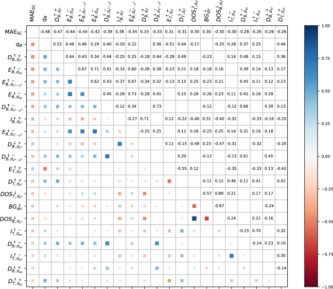
Figure 1 shows the twenty features most strongly correlated with MAE_SC, as well as their pairwise correlations. All of these top features are electronic and none of the structural features exhibits significant correlation with MAE_SC. Among these, thirteen are linked to TM_B and six to TM_T.

The color intensity and size of squares below the diagonal indicate the correlation strength between magnetic anisotropy energy obtained from self-consistent DFT calculations with SOC (MAE_SC) and system features from scalar-relativistic DFT, with exact numerical values provided above the diagonal. The first row and column represent correlations of each feature with MAE_SC, while the remaining elements show pairwise correlations between features. DOS denotes density of states at the Fermi level (E_F), D is the height of the first prominent peak in the DOS spectra, E represents its location on the energy axis, and I denotes integrated DOS using Eq. (8). The subscript refers to the position of TM atom (bottom or top) and an orbital type, and the superscript to the spin up/down direction. The sign indicates DOS below ( + ) and above ( − ) E_F. The direct bandgap is denoted by BG_dir, q_B is the Bader charge on the TM_B atom, and μ_T is the magnetic moment on the TM_T atom.

The Bader charge on the TM_B atom (q_B) shows the strongest correlation with MAE_SC, with a Spearman’s coefficient of −0.48, while the corresponding feature for the TM_T atom exhibits a much weaker correlation of 0.07. Although these dependencies are noticeable in Table S2, they do not represent a simple (inverse) linear relationship with MAE_SC (Table S1). The height of the first prominent peak in the spin-up DOS below the Fermi level (E_F) for TM_B (\({D}_{B,{d}_{{z}^{2}}}^{\uparrow +}\)), also shows a strong negative correlation with MAE_SC at ρ of −0.47. For the TM_T atom, this correlation is weaker at −0.31.

Figure 1 further reveals inter-correlations between DOS features of the TM_B atom above and below E_F, some of which align with PT-based orbital interaction rules for MAE^{34,35,36,37,38} (Table 1), for example pairs of DOS-related features, such as \({D}_{B,{d}_{xz}}^{\downarrow +}\)/\({D}_{B,{d}_{{x}^{2}-{y}^{2}}}^{\downarrow -}\), \({D}_{B,{d}_{xz}}^{\downarrow +}\)/\({D}_{B,{d}_{{x}^{2}-{y}^{2}}}^{\uparrow -}\), and \({D}_{B,{d}_{xz}}^{\downarrow +}\)/\({D}_{B,{d}_{xy}}^{\uparrow -}\). Conversely, \({D}_{B,{d}_{{z}^{2}}}^{\uparrow +}\)/\({D}_{B,{d}_{{x}^{2}-{y}^{2}}}^{\uparrow -}\) exhibit a inter-correlation coefficient of 0.44, but these states do not couple in a way that directly influences MAE. Moreover, none of the TM_T atom’s electronic features show mutual correlations that align with the PT-based coupling rules.

Among other features, the direct bandgap for spin-down electrons shows a moderate correlation (0.30), though this pattern does not generalize across all DFT-inspected systems, and for spin-up electrons, ρ is only 0.08, dropping below 0.05 for the indirect bandgap.

To broaden our analysis, we calculated additional correlation matrices, using Kendall’s τ coefficient (Fig. S1) for nonlinear correlations and Pearson’s coefficient r (Fig. S2) for linear correlations. Regardless of the statistical measure used—Spearman’s, Kendall’s, or Pearson’s—each approach is inherently limited, correlating MAE_SC with single features and neglecting the impact of feature combinations on MAE_SC. Consequently, the results provide only a simplified, univariate perspective on feature dependencies, likely overlooking the intricate, multi-feature interactions that impact MAE_SC.

To address these limitations, an ML model is developed with improved predictive capability and generalization for reliable MAE estimation, even in systems beyond the training set.

ML model for MAE prediction

The ML model is trained in a supervised manner, utilizing cost-effective SR-DFT calculations specified in the preceding section as input, while data from NCL DFT with SOC are used to generate correct outputs for training. Once trained, the model can predict MAE without requiring expensive NCL-SOC calculations, significantly enhancing computational efficiency.

Figure 2 a compares the MAEs predicted by the ML model with two baseline models—Multivariate Linear Regression (MLR) and Multivariate Lasso Regression (LASSO)—as well as with DFT-computed values. Cross-validation ensures predictions for all data points, with each inference made on unseen data, mitigating the risk of overfitting.

a Predictions of magnetic anisotropy energies (MAE) from a model trained on all features. b Predictions of MAE from a model trained on 25 selected features. Black dots and blue triangles represent Multivariate Linear Regression (MLR)-based predictions and Least Absolute Shrinkage and Selection Operator (LASSO)-based predictions, respectively, and red dots represent Machine Learning (ML)-based predictions. On both panels predictions for explicit substrates are denoted by green markers, with the shape indicating the method used. Most data points for MLR and LASSO are outside the plotting area (see Table 2 for the metrics). Histogram insets on both panels depict the distribution of prediction errors for the ML model (red), MLR (black), and LASSO (blue).

The ML model significantly outperforms both MLR and LASSO. The Root Mean Squared Error (RMSErr, Eq. (6)) for the ML model is nearly seven times smaller, and the Mean Absolute Error (MAErr, Eq. (7)) is over two times lower (Table 2). Additionally, the ML model achieves a determination coefficient (R²) greater than 0.8, indicating a strong fit and validating the model’s effectiveness. In contrast, MLR yields a negative R², indicating a poor fit and highlighting the inadequacy of simple regression for capturing the non-linear relationship involved. While LASSO performs better than MLR due to its embedded regularization, it still falls short, with RMSErr and MAErr nearly double those of the ML model.

The error distributions for all three models are shown in the inset of Fig. 2a. The ML model, leveraging cost-effective SR-DFT data, demonstrates high accuracy, with a mean absolute deviation of just 8.3 meV. In comparison, MLR and LASSO perform much worse, with some MAE predictions so inaccurate they are excluded from Fig. 2a for clarity (Fig. S3a). This highlights the necessity of more sophisticated and flexible methods, such as the boosting technique employed in our ML model.

Features selection

Including all 153 system features in the ML model could introduce irrelevant variables, potentially causing overfitting and adding unnecessary complexity. To address this, the Recursive Feature Elimination (RFE) algorithm⁴⁰ is applied in combination with SHapley Additive exPlanations (SHAP) values⁴¹ to evaluate feature importance. This iterative process continues until the optimal feature set is achieved (Fig. S4). Of the twenty-five selected features (Table 3), twenty-three are electronic properties, with only eight overlapping with those most strongly correlated with MAE_SC in Fig. 1. The remaining two features—the average surface–TM_B distance, h_sub, and the TM_B–TM_T bond length, d_len—are geometric descriptors.

Model performance metrics (Fig. S4) reveal that reducing the feature set from 153 to twenty-five not only simplifies the model but also improves its accuracy (Fig. 2b and S3b). While this reduction also enhances predictions made by MLR, bringing its performance closer to that of LASSO (Table 2), the ML approach continues to outperform both models. These findings highlight the limitations of linear models in capturing complex, multi-dimensional interactions impacting MAE. Conversely, the ML model utilizes the combined influence of twenty-five features beyond the additive effects typical of linear regression frameworks.

Additionally, a separate ML model trained on the same SR-DFT data and reduced feature set used for MAE inference is designed to predict the SOC energies (E_SOC) of the TM atoms in the dimers (Fig. S5). Figure 3 shows E_SOC values for TM_T and TM_B atoms in the dimers as predicted by the ML model compared to those computed using NCL-SOC DFT. With an R² of 0.86 for TM_B and 0.89 TM_T—exceeding the R² of 0.83 achieved for MAE prediction—this model exemplifies the robustness of our ML approach, adding confidence in its reliability for MAE predictions across a diverse set of systems, where SOC is a key factor.

a Predictions of spin-orbit coupling energies (SOC) for the bottom transition metal atom (TM_B). b Predictions of SOC energies for the top transition metal atom (TM_T). Black dots and blue triangles represent Multivariate Linear Regression (MLR)-based predictions and Least Absolute Shrinkage and Selection Operator (LASSO)-based predictions, respectively, and red dots represent Machine Learning (ML)-based predictions. Histogram insets on both panels depict the distribution of prediction errors for the ML model (red), MLR (black), and LASSO (blue).

Model generalization

The ML model, trained on SR-DFT data for OsPd, OsPt, IrPd, and IrPt dimers on both freestanding NSV-graphene and NSV-graphene with an implicit Ir(111) substrate, is evaluated for robustness and adaptability by predicting MAEs for systems on explicit substrates, including the metallic (111) surfaces and MgO(001) in their ground state (GS) geometries. For these configurations, all input features are derived directly from SR-DFT calculations, thus extending the model’s applicability to more complex systems.

The predictive performance of MLR and LASSO declines sharply for systems with explicit substrates, with many predictions falling well outside the range shown in Fig. 2b and R² values turning negative (Table 2, Fig. S3b). In contrast, while the ML model’s RMSErr and MAErr increase approximately threefold, it retains an R² of 0.42, indicating reasonable predictive power even under these challenging conditions.

These outcomes further reinforce the ML model’s adaptability to diverse material systems, while MLR and LASSO fail to generalize effectively, indicating that these simpler methods lack the complexity needed to handle the intricacies of the data.

Establishing whether the ML model accurately captures the physical principles underlying MAE is essential for developing reliable and interpretable frameworks, particularly given the inherent challenges of extrapolating beyond training datasets.

Second-order PT provides a valuable framework for understanding the origins of MAE, linking orbital interactions to fundamental system features. One of the primary factors driving MAE variations across systems is the position of the spin-up DOS peak associated with the d_yzd_xz orbitals located between the TM atoms (Fig. 4 and Figs. S8–S15). For instance, in OsPd@NSV, couplings between occupied/unoccupied spin-up/spin-down d_yzd_xz/\({d}_{xy}{d}_{{x}^{2}-{y}^{2}}\) states near E_F dominate the MAE_PT contributions (Fig. 4a, Table S4). Substrate interactions strengthen the Os–Pd bond, shifting the d_yzd_xz states to lower energies and reducing MAE_PT across all substrates (Table S1), as reflected by coupling 1b in Fig. 4b and Table 4. For OsPt@NSV, the spin-up d_yzd_xz states lie above E_F providing negative contributions to MAE_PT via couplings 9 and 10 in Fig. 4c and Table 4. Positive contributions arise primarily from couplings 5a and 7a, as well as interactions between spin-down \({d}_{{z}^{2}}\) and spin-up d_yzd_xz states. On MgO(001), the MAE_SC increases by 26% to 151 meV due to the spin-up d_yz DOS shifting below E_F, which diminishes negative contributions while leaving positive contributions largely unaffected (Fig. 4d). For IrPd@NSV, the primary contributions to MAE_PT stem from couplings between occupied spin-down \({d}_{xy}{d}_{{x}^{2}-{y}^{2}}\) states with their unoccupied \({d}_{{x}^{2}-{y}^{2}}{d}_{xy}\) counterparts, as well as interactions between occupied spin-up d_yzd_xz states and unoccupied spin-down \({d}_{{z}^{2}}\). Similar interactions contribute to MAE_PT on MgO(001) (Fig. S12). However, for IrPt@NSV, very low magnetic moments on the TM atoms leads to the negligible MAE_SC and MAE_PT (Table S2). On substrates, a magnetic moment of 1.4–1.8 μ_B is induced on Ir, primarily affecting the occupied spin-down degenerate \({d}_{xy}{d}_{{x}^{2}-{y}^{2}}\) states. Splitting these states introduces significant MAE_PT contributions (Fig. S13).

a OsPd dimer on defective graphene (OsPd@NSV), b OsPd@NSV with MgO(001) substrate, c OsPt@NSV, and d OsPt@NSV@MgO(001). The d-orbitals of the upper transition metal atom in the dimer (TM_T) are color-coded as yellow, blue, green, turquoise, and red for d_xy, d_yz, \({d}_{{z}^{2}}\), d_xz, and \({d}_{{x}^{2}-{y}^{2}}\) orbital. Arrows indicate orbital interactions with significant contributions to the magnetic anisotropy energy calculated using second-order perturbation theory (MAE_PT), with numerical labels corresponding to entries (ID) in Table 4.

To evaluate the ML model’s capacity to capture these physical interactions, PT-derived contributions are incorporated as an additional feature (Fig. S6). The model’s performance (RMSErr of 12.5, MAErr of 8.4, and R² of 0.83) is nearly identical with or without PT-derived input, indicating that the primary feature set already encapsulates the essential physics needed for accurate MAE predictions. However, when RFE-SHAP feature selection reduces the model to nine features, PT-derived contribution rank among the most relevant predictors. In this context, PT serves more as a validation of the ML model’s physical coherence, especially within simplified systems, rather than as a critical contributor to predictive accuracy.

Further analysis involved training a separate ML model to predict PT-derived contributions directly, excluding MAE_SC as a feature (Fig. S7). This model achieves an impressive R² of 0.95, surpassing the 0.83 obtained for direct MAE_SC predictions (Table 2). While this reinforces PT’s role in explaining key physical insights, its redundancy in enhancing the ML model’s performance highlights the strength of other descriptors in capturing the underlying physics.

For systems on explicit substrates, the inclusion of PT-derived contributions in the ML model results in a performance decline (RMSErr of 48.7, MAErr of 33.7, and R² of 0.19), likely due to redundancy and potential overfitting. This underscores the necessity of a broader feature set to predict MAE effectively in complex systems, a key strength of the current ML model, which captures substrate-specific descriptors beyond PT’s scope.

To test its generalizability, the ML model is applied to TM dimers on NSV-graphene not included in the training set—OsCo, IrCo, OsIr, IrIr—across all substrates (Table S1). Although predictive performance declines, the model successfully captures overall trends in MAE variation across substrates (Table S1). Moreover, deviations are as low as 7% and 8% for OsIr@NSV and OsCo@NSV on Ni(111), while increasing to 15% and 22% for OsCo@NSV and IrCo@NSV on Cu(111), exemplifying the model’s reasonable accuracy and trend fidelity (Table S1).

In conclusion, our CatBoost-based ML model significantly outperforms simpler approaches like Multivariate Linear Regression and Lasso Regression in predicting MAE across diverse systems. By capturing key dependencies, including SOC effects, that strongly influence magnetic anisotropy, the model extends beyond typical PT descriptors, offering deeper insights into atomic-scale anisotropy. While generalizability may be limited for systems that deviate significantly from the training set, expanding the descriptor space and refining the training process hold promise for further enhancing applicability. For instance, extending ML models to incorporate quantum multiplet effects represents an exciting direction for future work, potentially leading to a more comprehensive understanding of atomic-scale magnetic behavior. Ultimately, this work underscores the transformative potential of ML in pushing the boundaries of materials discovery and design.

Density-functional-theory calculations

All calculations were conducted using spin-polarized DFT within the Vienna ab-initio simulation package (VASP)^42,43,44,45. The exchange-correlation energy was evaluated using the generalized gradient approximation (GGA)⁴⁶, specifically the Perdew-Burke-Ernzerhof (PBE) functional⁴⁷. While PBE has been widely used for studying magnetic anisotropy, it is known that semi-local functionals may sometimes lead to inaccurate electronic and magnetic ground states, largely due to self-interaction errors^48,49,50. To address such limitations, orbital-dependent corrections can be introduced via hybrid functionals that mix Hartree-Fock and DFT exchange^51,52 or through a DFT + U approach incorporating an orbital-dependent on-site Coulomb repulsion U⁵³. However, prior investigations⁵⁴ have shown that applying hybrid functionals or GGA + U leads to only minor modifications in MAE predictions, as long as physically reasonable values of U are used. These findings suggest that our ML model, trained on PBE-level data, remains robust in capturing key trends in MAE across diverse systems. The projected augmented wave (PAW) method^55,56 was used to account for electron-ion interactions. Electron wavefunctions were expanded in plane waves with a 400 eV cutoff energy for both SR and NCL modes, a value previously established to ensure convergence for TM dimers in vacancy defects in the graphene monolayer^19,20. To handle partially occupied orbitals, a Gaussian smearing scheme with a width of 0.02 eV was applied. Self-consistent calculations continued until total energy changes were below 10⁻⁶ eV. Symmetry was disabled in all calculations to accurately capture the magnetic characteristics of the systems.

The geometry relaxations were initially performed at the Γ point of the Brillouin zone and then re-relaxed using a 2 × 2 × 1 k-point grid. However, for the final static calculations, a 6 × 6 × 1 k-point mesh was utilized to ensure accurate sampling of the reciprocal space. Due to the significant computational demands in the NCL mode, a 3 × 3 × 1 k-point mesh was employed for the initial MAE_SC calculations. Subsequently, systems exhibiting the highest MAE_SC values were selected for further analysis. For these systems, the NCL-SOC-DFT calculations were repeated using a denser 6 × 6 × 1 k-point mesh. In most cases, this refinement led to only minor changes in the MAE_SC values.

Magnetic anisotropy energies were obtained from NCL-SOC DFT^57,58,59,60. Due to their demanding nature, only static calculations were performed. MAE_SC was determined using the formula:

where E represents the total energy of the system with the initial magnetization aligned along the specified axis. The z-axis is defined as perpendicular to the graphene layer and parallel to the TM dimer bond. A positive MAE value indicates that the z-axis is the easy axis of magnetization. The contribution of interactions between d orbital pairs was calculated within the second-order PT framework^{34,35,36,37,38}.

For the five d-orbital-derived states per spin, the coupling between occupied and unoccupied states near E_F within the same spin channel is given by

For orbital interactions between opposite spin channels, the contribution is expressed as

Here, ξ is the SOC constant⁵⁴, o and u represent occupied and unoccupied states, E_u and E_o are their respective energies derived from the VASP-PROCAR file using a custom script, and L_z and L_x are angular momentum operators. Non-zero matrix elements are³⁴\(\langle {d}_{{x}^{2}-{y}^{2}}| {L}_{z}| {d}_{xy}\rangle =2\), \(\langle {d}_{xy}| {L}_{z}| {d}_{yz}\rangle =1\), \(\langle {d}_{xy}| {L}_{x}| {d}_{xz}\rangle =1\), \(\langle {d}_{{x}^{2}-{y}^{2}}| {L}_{x}| {d}_{yz}\rangle =1\), \(\langle {d}_{{z}^{2}}| {L}_{x}| {d}_{xz}\rangle =\sqrt{3}\), and \(\langle {d}_{{z}^{2}}| {L}_{x}| {d}_{yz}\rangle =\sqrt{3}\). Combining these terms, Equations (2) and (3) taken together, reduce to

where L_o,u is the orbital interaction contribution resulting from the combination of L_z and L_x (Table 1). The effect is inversely proportional to the energy distance of involved orbitals, making it sufficient to focus on states close to E_F. To avoid relying on an arbitrary cutoff energy difference, the full MAE_PT is calculated by including all states from the DFT calculations.

The contributions to overall MAE are calculated by analyzing all bands across all k-points, filtering out bands with zero contribution from the TM atoms as they have negligible impact on the MAE. For each spin combination, k-point (k), occupied band (o), unoccupied band (u), and TM atom, the MAE contribution is given by

where w(k) is the weight of the k-point (with all k-point weights summing to 1). s_m is the spin multiplier, set to + 1 if both states are in the same spin channel, and −1 if they are in opposite channels. The weights w(o_o) and w(o_u) reflect each orbital’s contribution within the bands, calculated as \(w({o}_{o})=\frac{c({o}_{o})}{c(tot)}\), where c(o_o) is the contribution of a specific orbital to the band and c(tot) is the sum of all orbital contributions across all atoms in the Wigner-Seitz cells. This value, usually less than 1, accounts for the fact that the Wigner-Seitz cell typically does not fully capture entire orbital contributions. w(o_u) is calculated in a similar manner.

To prevent unrealistically high contributions to MAE_PT due to near-zero denominators, a penalty energy (E_pen) is added to the denominator, with 0.1 eV determined as an optimal compromise.

When calculating MAE_PT using PT-derived contributions, it is also necessary to account for symmetry-based reductions (term s_r, see³⁴). Choosing the appropriate s_r value is non-trivial, especially for complex systems with slightly corrugated graphene sheets and multiple atomic species (like C, N, and TM atoms). In our systems, the best alignment with MAE_SC is achieved using s_r = 12.

Interatomic orbital couplings between TM_T and TM_B, representing molecular orbital interactions, are also considered. Here, MAE_PT would require division by an additional factor of 2 to account for these new contributions and avoid double-counting. While this adjustment improved PT’s predictive performance in some cases, it also increased discussion complexity. Consequently, the simplified model (excluding interatomic couplings) is used throughout the manuscript, except where ML-PT relationships are specifically discussed, with PT serving as an ML target value and being incorporated to enhance the ML model’s predictive capability.

Machine learning

To establish the relationship between MAE and structural and electronic parameters, various ML regression algorithms were tested. CatBoost³³, a state-of-the art gradient boosting regression tree algorithm, provided the best performance and was used in this study. Other algorithms, such as XGBoost and fully connected artificial neural networks, were also considered but yielded larger errors than CatBoost. Tree-based algorithms like CatBoost, inherently incorporating non-linear relationships between target and input features, are known to outperform neural networks in tabular data scenarios⁶¹.

Given the relatively small dataset, a five-fold cross-validation technique was used. The dataset was randomly partitioned into five non-intersecting subsets, with each subset serving as the test set once, while the remaining four were used for training. To illustrate, in each iteration, a specific fold (e.g., fold 1), was designated as the test set, while the remaining folds (2–5) were used for training. The model trained on folds 2–5 then predicted the MAE for the systems in fold 1. This process was repeated for all five folds, ensuring that each system was used exactly once as a test sample and four times as part of the training set. The models were trained on systems with implicit substrates, while systems with explicit substrates were excluded from the training process. Table S12 presents the R² metrics for each fold separately for models trained on the selected 25 features, whereas all other metrics reported in this paper are averages across all folds. All 806 systems (see below) considered in the manuscript are prediction systems, and results from training subsets are not reported. Additionally, a separate model was trained using the entire implicit-substrate dataset (without fold splitting) and used to predict MAE for systems with explicit substrates.

Multivariate Linear Regression (MLR) and Multivariate Lasso Regression (LASSO)—trained applying the same procedure—were used as benchmarks for comparison, which helped assess how much of the mapping between input features and MAE_SC can be modeled as simple linear relationship.

During the training process, the Root Mean Square Error (RMSErr)

served as the loss function. In the above the MAE_SC,i is the DFT-computed magnetic anisotropy energy of the i-th structure, while \({\widehat{MAE}}_{i}\) is the value estimated by the model. Additionally, the fit quality was evaluated using the Mean Absolute Error (MAErr)

The ML model was trained on SR-DFT data to identify system features correlated with MAE, derived from more expensive NCL-SOC calculations. The dataset comprised eight subsets, each corresponding to one dimer type (OsPd, OsPt, IrPd, or IrPt) deposited on either freestanding NSV-graphene or NSV-graphene constrained to the geometry resulting from interactions with the underlying Ir(111) substrate. Initially, each subset contained 112 geometric configurations, generated by selecting 14 distinct TM_B positions near the NSV defect and adding TM_T to create an upright dimer as well as five tilted configurations. Following geometric relaxations—where only the TM atoms were allowed to adjust along the z-axis—two additional structures were created for each relaxed upright dimer by shifting TM_T by ± 0.1 Å along the z-direction. NCL-SOC calculations were conducted on 896 structures in total, of which 90 were later discarded due to non-converged MAE_SC. The final dataset included 220 OsPd, 195 OsPt, 197 IrPd, and 194 IrPt dimers, totaling 806 configurations.

Each atomic configuration of a TM dimer on NSV-graphene was characterized by structural and electronic properties derived from SR-DFT calculations, serving as input features for the ML models. The more expensive NCL-SOC calculations were performed only to compute the MAE_SC. Thus, inference on unseen systems required only DFT-SR outputs.

Structural parameters included dimer bond length d_len, tilt angle relative to the surface normal, distance from the site of the missing carbon atom to the TM_B atom, and the vertical distance between NSV-graphene and the TM_B atom (h_sub).

System features associated with electronic properties encompassed the Bader charge on both the TM_B and TM_T atoms, calculated as the difference between the electron count from Bader analysis and the atom’s valence electrons, as well as the direct BG_dir and indirect BG_indir bandgaps for each spin channel.

Density-of-sates related features required vectorization before input into the ML model. Two methods were used, an integral-based and a peak-based approach.

In the integral method, partial DOS within ± L-width windows around E_F was integrated for each orbital j of atom k with spin orientation s = {↑, ↓}:

In practice, j corresponds to one of five d-orbitals, \(j\in \{{d}_{xy},{d}_{yz},{d}_{{z}^{2}},{d}_{xz},{d}_{{x}^{2}-{y}^{2}}\}\), and k denotes one of the two dimer adatoms, with k = B for TM_B and k = T for TM_T. Here, the integration limit was set to L = 1.0 eV, though other values (L = 0.5 eV and L = 2.0 eV) were tested with similar results.

The peak-based method identified prominent peaks in the DOS spectra near E_F, with each peak characterized by its location and height. This approach is inspired by the PT-based analyses available in the literature that relates the MAE with the DOS spectra peaks^35,36,37,38. Using the same notation as in Eq. (8), \({D}_{k,j}^{s,+}\) (\({D}_{k,j}^{s,-}\)) denotes height of the first prominent peak below (above) E_F for TM atom k, orbital j and spin s, while \({E}_{k,j}^{s,+}\) (\({E}_{k,j}^{s,-}\)) represent the peak location on the energy axis.

Each system was thus characterized by forty features for the integral-based method, eighty for the peak-based method, and an additional twenty features representing spin and orbital-resolved DOS of each TM atom at E_F (\(DO{S}_{k,j}^{s}({E}_{F})\)). The workfunction ϕ of the system and the magnetic moment μ_B (μ_T) of each bottom (top) TM dimer atom was also included, resulting in 153 features per system. Notably, none of these features directly identified the atomic types constituting the dimer.

The RFE algorithm⁴⁰ along with SHAP values⁴¹ were used as importance measures determining which features had the strongest impact on the ML model’s predictions. The Shapley values might be either negative or positive and hence it is an absolute value of the Shapley value that describe the relative importance of given feature for the model⁶². SHAP, based on coalition game theory, calculates Shapley values to distribute contributions among input features fairly. The overall importance of each feature was represented by the average absolute Shapley value across all data points.

The codebase and datasets associated with our ML model are available at https://github. com/RafalTopolnicki/MLforMagneticAnisotropyEnergy.

Authors and Affiliations

1. Regional Centre of Advanced Technologies and Materials, Czech Advanced Technology and Research Institute (CATRIN), Palacký University Olomouc, Olomouc, Czech Republic

   Jan Navrátil, Michal Otyepka & Piotr Błoński

2. Department of Physical Chemistry, Faculty of Science, Palacký University Olomouc, Olomouc, Czech Republic

   Jan Navrátil

3. Dioscuri Center in Topological Data Analysis, Institute of Mathematics, Polish Academy of Sciences, Warsaw, Poland

   Rafał Topolnicki

4. Institute of Experimental Physics, University of Wrocław, Wrocław, Poland

   Rafał Topolnicki

5. IT4Innovations, VŠB–Technical University of Ostrava, Ostrava-Poruba, Czech Republic

   Michal Otyepka & Piotr Błoński

Contributions

P.B. conceived the study, coordinated the project, and drafted the manuscript. J.N. executed and analyzed the DFT calculations. R.T. designed and analyzed the ML model. M.O. contributed to the discussion of data and assisted in manuscript drafting. All authors contributed to data analysis and discussion, writing, reviewing, and editing, and have read and approved the final manuscript.

Corresponding authors

Correspondence to Rafał Topolnicki or Piotr Błoński.

Competing interests

The authors declare no competing interests.

Open Access This article is licensed under a Creative Commons Attribution 4.0 International License, which permits use, sharing, adaptation, distribution and reproduction in any medium or format, as long as you give appropriate credit to the original author(s) and the source, provide a link to the Creative Commons licence, and indicate if changes were made. The images or other third party material in this article are included in the article’s Creative Commons licence, unless indicated otherwise in a credit line to the material. If material is not included in the article’s Creative Commons licence and your intended use is not permitted by statutory regulation or exceeds the permitted use, you will need to obtain permission directly from the copyright holder. To view a copy of this licence, visit http://creativecommons.org/licenses/by/4.0/.

Reprints and permissions

References

Andrae, A. S. New perspectives on internet electricity use in 2030. Eng. Appl. Sci. Lett. 3, 19–31 (2020).
Freitag, C. et al. The real climate and transformative impact of ICT: A critique of estimates, trends, and regulations. Patterns 2, 100340 (2021).
Dong, Y., Sun, F., Ping, Z., Ouyang, Q. & Qian, L. DNA storage: research landscape and future prospects. Natl Sci. Rev. 7, 1092–1107 (2020).
Gambardella, P. et al. Giant Magnetic Anisotropy of Single Cobalt Atoms and Nanoparticles. Science 300, 1130–3 (2003).
Rau, I. G. et al. Reaching the magnetic anisotropy limit of a 3 d metal atom. Science 344, 988–992 (2014).
Baumann, S. et al. Electron paramagnetic resonance of individual atoms on a surface. Science 350, 417–420 (2015).
Natterer, F. D., Donati, F., Patthey, F. & Brune, H. Thermal and Magnetic-Field Stability of Holmium Single-Atom Magnets. Phys. Rev. Lett. 121, 027201 (2018).
Singha, A. et al. Engineering atomic-scale magnetic fields by dysprosium single atom magnets. Nat. Commun. 12, 4179 (2021).
Novoselov, K. S. Electric Field Effect in Atomically Thin Carbon Films. Science 306, 666–669 (2004).
Baltic, R. et al. Superlattice of Single Atom Magnets on Graphene. Nano Lett. 16, 7610–7615 (2016).
Shick, A. & Denisov, A. Magnetism of 4f-atoms adsorbed on metal and graphene substrates. J. Magn. Magn. Mater. 475, 211–215 (2019).
Shick, A. B., Kolorenč, J., Denisov, A. Y. & Shapiro, D. S. Magnetic anisotropy of a Dy atom on a graphene/Cu(111) surface. Phys. Rev. B 102, 064402 (2020).
Lin, Y.-C., Teng, P.-Y., Chiu, P.-W. & Suenaga, K. Exploring the Single Atom Spin State by Electron Spectroscopy. Phys. Rev. Lett. 115, 206803 (2015).
Dyck, O. et al. Doping of Cr in Graphene Using Electron Beam Manipulation for Functional Defect Engineering. ACS Appl. Nano Mater. 3, 10855–10863 (2020).
Gan, Y., Sun, L. & Banhart, F. One- and Two-Dimensional Diffusion of Metal Atoms in Graphene. Small 4, 587–591 (2008).
Fei, H. et al. Microwave-Assisted Rapid Synthesis of Graphene-Supported Single Atomic Metals. Adv. Mater. 30, 1802146 (2018).
Xia, B. et al. Realization of “single-atom ferromagnetism” in graphene by Cu-N 4 moieties anchoring. Appl. Phys. Lett. 116, 113102 (2020).
Dyck, O. et al. Doping transition-metal atoms in graphene for atomic-scale tailoring of electronic, magnetic, and quantum topological properties. Carbon 173, 205–214 (2021).
Navrátil, J., Błoński, P. & Otyepka, M. Large Magnetic Anisotropy in OsIr Dimer Anchored in Defective Graphene. Nanotechnology 32, 230001 (2021).
Navrátil, J., Otyepka, M. & Błoński, P. OsPd bimetallic dimer pushes the limit of magnetic anisotropy in atom-sized magnets for data storage. Nanotechnology 33, 215001 (2022).
Langer, R. et al. Graphene Lattices with Embedded Transition-Metal Atoms and Tunable Magnetic Anisotropy Energy: Implications for Spintronic Devices. ACS Appl. Nano Mater. 5, 1562–1573 (2022).
Néel, L. Théorie du trai^nage magnétique des ferromagnétiques en grains fins avec application aux terres cuites. Annales de. g.éophysique 5, 99–136 (1949).
Soumyanarayanan, A., Reyren, N., Fert, A. & Panagopoulos, C. Emergent phenomena induced by spin-orbit coupling at surfaces and interfaces. Nature 539, 509–517 (2016).
Gao, L., Guest, J. R. & Guisinger, N. P. Epitaxial Graphene on Cu(111). Nano Lett. 10, 3512–3516 (2010).
Gaddam, S. et al. Direct graphene growth on MgO: origin of the band gap. J. Phys.: Condens. Matter 23, 072204 (2011).
Zhao, W. et al. Graphene on Ni(111): Coexistence of Different Surface Structures. J. Phys. Chem. Lett. 2, 759–764 (2011).
Błoński, P. & Hafner, J. Pt3 and pt4 clusters on graphene monolayers supported on a Ni(111) substrate: Relativistic density-functional calculations. J. Chem. Phys. 137, 34107 (2012).
Achilli, S. et al. Surface states characterization in the strongly interacting graphene/Ni(111) system. N. J. Phys. 20, 103039 (2018).
Dedkov, Y., Zhou, J., Guo, Y. & Voloshina, E. Easy Approach to Graphene Growth on Ir(111) and Ru(0001) from Liquid Ethanol. Adv. Mater. Interfaces 10, 2300468 (2023).
Zheng, L. et al. N-doped graphene-based copper nanocomposite with ultralow electrical resistivity and high thermal conductivity. Sci. Rep. 8, 9248 (2018).
Pétuya, R. & Arnau, A. Magnetic coupling between 3d transition metal adatoms on graphene supported by metallic substrates. Carbon 116, 599–605 (2017).
Xia, W. et al. Accelerating the discovery of novel magnetic materials using machine learning-guided adaptive feedback. PNAS 119, e2204485119 (2022).
Prokhorenkova, L., Gusev, G., Vorobev, A., Dorogush, A. V. & Gulin, A. CatBoost: unbiased boosting with categorical features. http://arxiv.org/abs/1706.09516 (2019).
Wang, D.-s, Wu, R. & Freeman, A. J. First-principles theory of surface magnetocrystalline anisotropy and the diatomic-pair model. Phys. Rev. B 47, 14932–14947 (1993).
Daalderop, G. H. O., Kelly, P. J. & Schuurmans, M. F. H. Magnetic anisotropy of a free-standing Co monolayer and of multilayers which contain Co monolayers. Phys. Rev. B 50, 9989–10003 (1994).
Zhang, Y., Wang, Z. & Cao, J. Prediction of magnetic anisotropy of 5d transition metal-doped g-c3n4. J. Mater. Chem. C. 2, 8817–8821 (2014).
Whangbo, M.-H., Gordon, E. E., Xiang, H., Koo, H.-J. & Lee, C. Prediction of Spin Orientations in Terms of HOMO-LUMO Interactions Using Spin-Orbit Coupling as Perturbation. Acc. Chem. Res. 48, 3080–3087 (2015).
Zhou, J., Wang, Q., Sun, Q., Kawazoe, Y. & Jena, P. Giant magnetocrystalline anisotropy of 5d transition metal-based phthalocyanine sheet. Phys. Chem. Chem. Phys. 17, 17182–17189 (2015).
Zhong, X. et al. Explainable machine learning in materials science. npj Computational Mater. 8, 204 (2022).
Guyon, I., Weston, J., Barnhill, S. & Vapnik, V. Gene Selection for Cancer Classification using Support Vector Machines. Mach. Learn. 46, 389–422 (2002).
Lundberg, S. & Lee, S.-I. A Unified Approach to Interpreting Model Predictions. https://arxiv.org/abs/1705.07874 (2017).
Kresse, G. & Hafner, J. Ab initio molecular dynamics for liquid metals. Phys. Rev. B 47, 558–561 (1993).
Kresse, G. & Hafner, J. Ab initio molecular-dynamics simulation of the liquid-metal-amorphous-semiconductor transition in germanium. Phys. Rev. B 49, 14251–14269 (1994).
Kresse, G. & Furthmüller, J. Efficiency of ab-initio total energy calculations for metals and semiconductors using a plane-wave basis set. Comput. Mater. Sci. 6, 15–50 (1996).
Kresse, G. & Furthmüller, J. Efficient iterative schemes for ab initio total-energy calculations using a plane-wave basis set. Phys. Rev. B 54, 11169–11186 (1996).
Perdew, J. P. et al. Atoms, molecules, solids, and surfaces: Applications of the generalized gradient approximation for exchange and correlation. Phys. Rev. B 46, 6671–6687 (1992).
Perdew, J. P., Burke, K. & Ernzerhof, M. Generalized Gradient Approximation Made Simple. Phys. Rev. Lett. 77, 3865–3868 (1996).
Droghetti, A., Pemmaraju, C. D. & Sanvito, S. Predicting d 0 magnetism: Self-interaction correction scheme. Phys. Rev. B 78, 140404 (2008).
Zhong, X., Rungger, I., Zapol, P. & Heinonen, O. Electronic and magnetic properties of T i 4 O 7 predicted by self-interaction-corrected density functional theory. Phys. Rev. B 91, 115143 (2015).
Shinde, R., Yamijala, S. S. R. K. C. & Wong, B. M. Improved band gaps and structural properties from Wannier-Fermi-Löwdin self-interaction corrections for periodic systems. J. Phys.: Condens. Matter 33, 115501 (2021).
Heyd, J., Scuseria, G. E. & Ernzerhof, M. Hybrid functionals based on a screened Coulomb potential. J. Chem. Phys. 118, 8207–8215 (2003).
Heyd, J. & Scuseria, G. E. Assessment and validation of a screened Coulomb hybrid density functional. J. Chem. Phys. 120, 7274–7280 (2004).
Anisimov, V. I., Zaanen, J. & Andersen, O. K. Band theory and Mott insulators: Hubbard U instead of Stoner I. Phys. Rev. B 44, 943–954 (1991).
Błoński, P. & Hafner, J. Magnetic anisotropy of transition-metal dimers: Density functional calculations. Phys. Rev. B 79, 224418 (2009).
Kresse, G. & Joubert, D. From ultrasoft pseudopotentials to the projector augmented-wave method. Phys. Rev. B 59, 1758–1775 (1999).
Blöchl, P. E. Projector augmented-wave method. Phys. Rev. B 50, 17953–17979 (1994).
Kleinman, L. Relativistic norm-conserving pseudopotential. Phys. Rev. B 21, 2630–2631 (1980).
MacDonald, A. H., Picket, W. E. & Koelling, D. D. A linearised relativistic augmented-plane-wave method utilising approximate pure spin basis functions. J. Phys. C: Solid State Phys. 13, 2675–2683 (1980).
Hobbs, D., Kresse, G. & Hafner, J. Fully unconstrained noncollinear magnetism within the projector augmented-wave method. Phys. Rev. B 62, 11556–11570 (2000).
Marsman, M. & Hafner, J. Broken symmetries in the crystalline and magnetic structures of γ-iron. Phys. Rev. B 66, 1–13 (2002).
Grinsztajn, L., Oyallon, E. & Varoquaux, G. Why do tree-based models still outperform deep learning on tabular data? arXiv. https://arxiv.org/abs/2207.08815 (2022).
Lundberg, S. M., Erion, G. G. & Lee, S.-I. Consistent individualized feature attribution for tree ensembles. https://arxiv.org/abs/1802.03888 (2019).
Acknowledgements
The work was supported by the project TECHSCALE (CZ.02.01.01/00/22_008/0004587) via the Operational Programme Johannes Amos Comenius and REFRESH –Research Excellence For REgion Sustainability and High-tech Industries (CZ.10.03.01/00/22_003/0000048) via the Operational Programme Just Transition. The support by the Ministry of Education, Youth and Sports of the Czech Republic through the e-INFRA CZ (ID:90254) is gratefully acknowledged. J.N. acknowledges the support from Palacký University Olomouc (project IGA_PrF_2025_003). P.B. acknowledges the Visiting Professors Programme at the University of Wroclaw within the Initiative of Excellence –Research University. R.T. acknowledges the support of the Dioscuri program initiated by the Max Planck Society, jointly managed with the National Science Centre (Poland), and mutually funded by the Polish Ministry of Science and Higher Education and the German Federal Ministry of Education and Research. We gratefully acknowledge Poland’s high-performance Infrastructure PLGrid ACK Cyfronet AGH for providing computer facilities and support within computational grant no plgheasc2.
Ethics declarations