Differentiability of voice disorders through explainable AI

Different types of pathology can affect the voice. Voice disorders result from a pathological process caused by anatomical, functional or paralytic factors. Voice production is affected by physiological, auditory, aerodynamic, acoustic and perceptual aspects¹.

Types of pathology can be grouped into three main categories for the dataset used in this study^2,3:

• Hyperkinetic dysphonia is a common condition, particularly among people in voice-intensive professions. Muscular hypercontraction of the pneumo-phonic apparatus makes the voice shrill and laboured. As a result, frequency modulation is reduced. More tiring phonation and altered respiratory dynamics are caused by high glottic resistance to expiratory airflow. Several diseases fall into this category: vocal cord nodules, chorea, rigid vocal cords, Reinke’s oedema, polyps and prolapse.

• Hypokinetic dysphonia is characterised by a reduction in vocal cord adduction during the respiratory cycle, resulting in obstruction of airflow through the larynx. A weak, breathless voice results from incomplete closure of the vocal folds. In this category of illness, the voice improves with increasing vocal intensity. Incorrect use of the voice may therefore be observed. Several conditions fall into this category: chordal groove dysphonia, presbiphonia, adduction deficit, conversion dysphonia, laryngitis, vocal fold paralysis, glottic insufficiency, and extraglottic air leakage.

• Reflux laryngitis: reflux of gastric acid into the oesophagus can cause inflammation of the larynx. Alongside symptoms that may be less or more pronounced, such as pharyngitis or a dizzy asthmatic cough, the most common symptom is chronic hoarseness.

The medical expert generally performs a laryngoscopy, diagnostic techniques used generally in phoniatry. This enables the anatomical structure of the vocal folds and any damage to them to be visualised. Through a phoniatric medical examination, the doctor diagnosed the presence or absence of a voice disorder^2,4. This invasive analysis is useful for observing morphological and functional changes in the vocal tract. Another important test for assessing the characteristic parameters extracted from the speech signal is the acoustic analysis, making it possible to estimate the state of health of the voice². An interdisciplinary approach to assessment is necessary for the diagnosis and treatment of voice disorders¹. To assess vocal health, various acoustic parameters need to be measured⁵. We are going to carry out the acoustic analysis using deep learning methods. Designing a highly promising new explicable diagnostic system using artificial intelligence will make it possible to characterise the patient’s vocal sound without laryngoscopy and to understand the characteristics used by the artificial network.

Due to natural disasters such as earthquakes, floods, epidemics such as Covid-19 and wars, humanity needs fast, easy and automatic healthcare solutions, and if necessary in a non-presence setting, i.e. by teleconsultation. Decision support systems can be used to meet these needs. Clinical decision support systems (CDSS) are computerised systems that are being used for a variety of purposes to improve healthcare: therapeutic planning and diagnostics, screening and prevention, drug decision-making, etc.⁶.

To design a CDSS, the data must be processed in a manner that is adapted to it. In this work, the sounds of pathological and non-pathological voices will be divided into time series which will be transformed into Mel Spectrograms, a logarithmic frequency spectrum on the Mel scale providing an important time–frequency representation of the audio signals⁷. When Mel Spectrogram’s two-dimensional images are presented to convolution networks pre-trained with audio data, very high process efficiency is achieved^8,9. The OpenL3 network^7,10 is a proven artificial network for classifying audio data^7,10.

The ontological identification of a class determined by specific properties can shed light on the complexity of classification¹¹. In this regard, a good CDSS should provide automatic decision support as part of the clinician’s workflow¹² and should provide explanations of the computerised decision. It is essential that clinicians using CDSS systems do not place blind trust⁶ and understand the reasons for the automatic decision. Explainable Decision Support Systems (XDSS) provide an in-depth understanding of the decision-making process leading to the development of decision support systems¹³. In this study, we therefore propose a new system architecture for analysing pathological speech in order to perform intelligent, explainable and potentially scalable speech diagnostics.

Firstly, a study of previous works will be reviewed in order to determine the problematic of this work. Lopes et al., using data from 279 patients, were able to obtain an accuracy of 83.5% for the prediction of subjects with voice disorders and healthy subjects. They used acoustic measurements of mean values and standard deviation (SD) of fundamental frequency, jitter, shimmer and glottal excitation to noise¹. Verde et al., using the Saarbrücken Voice Database (SVD), Massachusetts Eye and Ear Infirmary database (MEEI) and VOice ICar fEDerico II (VOICED) datasets, windowed at 10 ms, obtained 77% accuracy using the fundamental frequency among others (characteristic parameters such as jitter shimmer, and Harmonic to Noise Ratio) and one-way ANOVA (Statistical methods)¹⁴. In their work on the SVD dataset, Barbon et al. obtained the best F1score result, which was 94.3% for the 6-class classification (Healthy, Vox Senilis, Central Laryngeal Motion Disorder, Dysphonia, Laryngitis, Reinke’s Edema)¹⁵. With the same number of classes from the same dataset, Dişken achieved 99.4% accuracy¹⁶. Ur Rehman et al. have carried out an interesting study using the SVD and MEEI. They obtained up to 99.78% accuracy with machine learning methods⁵. The literature on the VOICED dataset is summarised in Table 1.

Work carried out with convolution networks pre-trained with audio data has proved their effectiveness^8,9. Explainability techniques are then added to the model to clarify the process of this performance and to gather more information on the important features of the dataset^17,18,19. Jegan and Jayagowri²⁰ carried out the classification work on the SVD, Arabic Voice Pathology Database (AVPD) and VOICED datasets, obtaining 1.02% more accuracy than previous work, using XAI with the Grad-CAM technique (Table 1). Occlusion Sensitivity is a method that provides explainability maps with appreciable resolution⁸.

The research carried out to date on the non-invasive detection of disordered voices has considerably advanced the field. They have used machine learning and deep learning techniques using the characteristics of the data. On the SVD dataset, with 687 samples and data augmentation, 6 groups were classified using deep learning techniques by training from scratch on 100 epochs. A maximum accuracy of 99.4% was achieved¹⁶. To obtain such a result, the number of batches and epochs is high and this increases the processing time. To summarise, binary classification achieved an accuracy value of 99% by Muraleedharan et al. and Wang et al. using different methods (Table 1)^29,33. Wahengbam et al.²⁵ using the VOICED dataset, for a 4-class classification, obtained 97.7% accuracy. These results remain very high, but there is no XAI analysis. Jegan and Jayagowri²⁰ classified three different datasets and used the Grad-CAM technique (Table 1). This work does not include multiclass classification and does not use XAI averaged over all correctly identified and classified images. In this study, Occlusion Sensitivity, method that provides explainability maps with appreciable resolution, will be used⁸.

This literature review is highly motivating for Explainable Artificial Intelligence (XAI) work on a dataset that has not obtained a remarkable accuracy value with the classification of 7 pathologies and healthy subjects.

In our work, we will use 2D images of Mel Spectrogram on the OpenL3 artificial network, using a transfer learning technique. We will use a limited amount of data over a short period of time for 8 classes in order to obtain the classification result with a short processing time. In addition, in this study the Occlusion Sensitivity explainability technique was used to understand the behaviour of the network during training. Obtaining an image from the averaging of all the Occlusion Sensitivity maps and comparing these maps will enable us to understand the spatio-temporal characteristics of the disordered voices. Comparing these maps will also allow us to see the non-apparent and non-obvious differences between classes, which are used by the model for classification. In the end, by highlighting the differentiability of the classes, we will obtain an explainable decision process (computer-aided diagnosis system) on the different disordered voices simply by using the recorded voices of the patients.

The VOice ICar fEDerico II (VOICED) dataset of healthy and pathological voices is publicly available on physionet.org. The data set consists of 208 healthy and pathological voices. These voices were collected during a clinical study carried out in accordance with the guidelines of the Società Italiana di Foniatria e Logopedia medical protocol and the declaration Standard Protocol Items: Recommendations for Interventional Trials. The database has been realized in a clinical study during 2016 and 2017 by the “Institute of High Performance Computing and Networking of the National Research Council of Italy (ICAR-CNR)” and the Hospital University of Naples “Federico II”. Recording study has been approved by the Federico II University Ethics Committee².

Adults aged between 18 and 70 who did not suffer from diseases such as upper respiratory tract infections or neurological disorders met appropriate inclusion criteria. There is a prevalence of disordered voices (150) compared to healthy ones (58). In detail, there were 73 male and 135 female participants. We do not consider the patient’s gender or age for inclusion in the work. Information on the participant’s lifestyle, such as data on voice use, smoking and alcohol abuse, eating habits, hydration habits and on previous or concomitant illnesses that could be related to voice disorders is not also included².

The medical expert performed laryngoscopy using the Henke Sass Wolf 6.0 mm autoclavable 70° rigid model laryngoscope and the 2.8 mm flexible model was used to perform laryngoscopy through the nose. Following the phoniatric medical examination, the doctor diagnosed the presence or absence of a voice disorder.

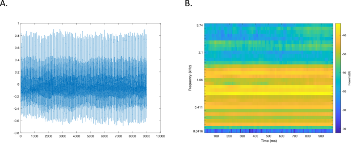
For each subject, a 5 s recording of the vowel/a/and the medical diagnosis formed the database. All the samples were recorded in a quiet room (< 30 dB background noise) that was not too dry. The microphone of a mobile device, a Samsung Galaxy S4, Android version 5.0.1, is used for recordings. It was held at a distance of about 20 cm from the patient and at an angle of about 45°. All recordings, sampled at 8000 Hz and with 32-bit resolution, were saved in. txt format (Fig. 1).

The vocal sound /a/ over one second of a patient with hyperkinetic dysphonia. (A) is the time signal over one second (8000 points per second). (B) is the Mel Spectrogram of the time signal in (A).

To eliminate any noise accidentally added during acquisition, each recording was filtered using a FIR filter. One method of designing an FIR filter is the windowing technique. By using a Hanning window, a low-pass FIR filter can be realised³⁴. The Hanning filter is expressed by the Eq. (1):

where x(n) and y(n) are the input and the output signal respectively and d is the normalization factor. The d value is empirically 2.

The dataset contains recordings of voices affected by different types of pathology: Hyperkinetic dysphonia, Hypokinetic dysphonia, reflux laryngitis vocal fold nodules, prolapse, glottic insufficiency et vocal fold paralysis. With the healthy class, we have a total of 8 classes to process. The operating principle is shown in Fig. 2.

Principle of voice pathology detection and differentiation. Created in BioRender⁴⁰.

There are 5 participant vocal sounds from the healthy and disordered voices, each lasting 5 s without any interruption. Each sound from the 8 classes was divided into 250 ms segments with an overlap of 125 ms. 36 images per sound were therefore generated. The first 1000 points are not used. This corresponds to 125 ms from the start of the unused time series.

The sounds are pre-processed by dividing them into 250 ms sequences with a 125 ms overlap. Each sequence is transformed into a Mel spectrogram. Models based on deep learning learn to recognise the characteristics of these Mel spectrograms of audio signals. The Mel spectrogram is a logarithmic frequency spectrum on the Mel scale, which approximates the perception of sound by the human ear⁷ and provides a time–frequency representation of sounds. The conversion from frequency to Mel scale is calculated by Formula (2), in relative to the frequency f^8,35,36. The formula is applied over a 250 ms window with a sampling frequency of 8000 Hz.

For classification, transfer learning was used, which involves fine-tuning the deep network³⁵. The pre-trained networks OpenL3¹⁰, Yamnet³⁷, VGGish³⁸ have been used. For each classification test, a cross-validation with k = 5 was applied. No data augmentation techniques were used. 70% of the data was used to train the model and the remaining 30% to test it. Accuracy, precision (on the confusion matrix), recall/sensitivity and the value of the area under the curve were taken into account to assess the performance^35,39.

To better understand the behaviour of the deep neural network and explain the reasons for the strengths and limitations of the features used, we can rely on the concept of Explainable Artificial Intelligence (XAI). The explainability method OcclusionSensitivity may be suitable for seeing the workings of the neural network in detail^8,35. The occlusion sensitivity technique uses an occlusion mask to disrupt the input. For a given class, the variation in the probability score is measured as the mask moves across the image⁴⁰.

We used a method of differentiation between classes by comparing the mean of the OcclusionSensistivity map. As the images in Fig. 4C are similar, the 2D cross-class correlation coefficients are calculated and presented in Fig. 5. The correlation coefficients of the images are calculated using formula (3)⁴⁰.

where \(\overline{A }\) is the average XAI maps of one class and where \(\overline{B }\) is the average XAI maps of another class.

The work was carried out on an Apple MacBook M2 Pro, with 16 GB of memory, a total number of 12 cores and a 19-core grafics processor, using Matlab 2024a.

There are 5 participant vocal sounds of 5 s for each class. Each sound provides 36 images over a 250 ms audio sequence. The prediction work in the classification is therefore done on 8 classes, with 36 × 5 × 8 (1440) 2D Mel Spectrogram images in total. For each class, 126 (70% of the total of 180 images per class) images were used for training, and 54 (30% of the total of 180 images per class) images were used for the test process.

The pre-trained CNN networks, OpenL3, Yamnet and VGGish, were used to evaluate classification performance. To evaluate the results, accuracy, recall/sensitivity and precision (on the confusion matrix) and the Area Under the Curve (AUC) value (with the ROC-receiver operating characteristic curve) were considered. A value of k = 5 was used for cross-validation.

Table 2 shows the accuracy values of the 3 pre-trained artificial networks (OpenL3, YAMNET, VGGish) together with the time taken for fine-tuning. OpenL3 remains the best performing network in terms of accuracy (99.44%), while YAMNET is the fastest (107 s) with 94.36% of accuracy. In addition, the confusion matrices and ROC curves are shown in Fig. 3 to give more detail on the classification performance of the eight classes. The accuracy of VGGish is 95.34% for a process that lasted 408 s.

Results for voice classification based on fine-tuning of OpenL3, YAMNET and VGGish. These results concern a single test without cross-validation. Eight classes are presented: Glottic Insufficiency, Hyperkinetic Dysphonia, Hypokinetic Dysphonia, Prolapse, Reflux Laryngitis, Vocal Fold Nodules, Vocal Fold Paralysis and Healthy. (A) The confusion matrices show the actual classes (rows) and the predicted classes (columns). The diagonal cells show the correctly classified observations. The measures shown at the bottom, in dark blue, are called precision. The measures on the right, shown in dark blue are called recall or sensitivity (false negative rates are in light blue). (B) ROC curves (different colours) and AUC values for the eight classes.

According to Fig. 3, for the 3 networks, the Glottic Insufficiency class ranked the lowest. For OpenL3, at worst, the precision of Glottic Insufficiency class was 98.2% and the recall of Vocal Fold Paralysis class was 98.1%. For Yamnet, the Prolapse class was also the worst classified. For VGGish, the Hypokinetic Dysphonia class was also the lowest scoring. The AUC value was lowest for Vocal Fold Paralysis. For VGGish, at worst, the precision of Hypokinetic Dysphonia class was 91.4% and the recall of Glottic Insufficiency, Hyperkinetic Dysphonia and Prolapse classes was 92.6%. Nevertheless, the AUC values for the 3 networks and for all the classes remain very high.

As OpenL3 is the best performing of the three networks in terms of accuracy, XAI’s work will be based on the OpenL3 model. For eight classes, Fig. 4 presents.

• examples of PCG Mel Spectrograms (Fig. 4A),

• XAI occlusionSensitivity map from one correctly classified image on origine image (Fig. 4B) showing areas/features used to correct classification,

• average images of XAI maps (Fig. 4C) showing the areas most used on average,

• standard deviation images of XAI maps (Fig. 4D)

• difference of averaged images according to the Fig. 4C (E). The classes to be compared were selected according to Fig. 5.

(A) Examples of voice Mel Spectrograms with Glottic Insufficiency, Hyperkinetic Dysphonia, Hypokinetic Dysphonia, Prolapse, Reflux Laryngitis, Vocal Fold Nodules, Vocal Fold Paralysis, HealthyThe graphical representation has the time (250 ms) as the abcissa and the Mel frequency (in kHz) as the ordinate. On the right-hand side of the image (from blue to yellow for the lowest to highest intensity) the intensity is shown. (B) XAI occlusionSensitivity map from correctly classified image for eight classes on origine image. The red areas mark the zones used by the model to make the related classification. (C) Average images of XAI maps + origine image (B) for eight classes. (D) Standard Deviation images of XAI maps + origine image (B) for eight classes. When the SD is low, the colour of the zone is green, when the SD is high, the colour of the zone is pink. (E). Inter-class differentiability maps. Difference in the comparison of averaged images according to the (C) The white zones mark the differences. The comparisons were chosen on the basis of the table containing the 2D correlation coefficients in Fig. 5.

2D correlation coefficient between classes. On the diagonal, as the same images are compared, the coefficient is equal to 1. Similar images with a coefficient value close to 0.7 and above are considered to assess the difference. The closer to value 1, the darker the green color.

In Fig. 4A, we can see examples of voice Mel Spectrograms and from these examples, it’s easy to see that it can be difficult to identify images that look like the human eye.

Figure 4B shows examples of the XAI occlusionSensitivity map on origine image from correctly classified images. The red areas mark the zones used by the model to make the related classification. The convolution network generally used the high intensity frequencies of the Mel spectrograms to correctly classify the cases.

In this study, to see the most used areas, we took the average image of all the OcclusionSensitivity maps. The resulting images are shown in Fig. 4C. These images show the overall difference in pathologies used by the deep learning model. Overall, the time variable does not influence the Mel Spectrograms and the 0–1.5 kHz frequency band is generally used. The priority frequencies are shown below for each class.

• Glottic Insufficiency: 2 frequencies are given priority, 400 Hz and 900 Hz. Frequencies around 40 Hz are not used.

• Hyperkinetic Dysphonia: A wide band around 700 Hz and 100 Hz are dominant.

• Hypokinetic Dysphonia A band over 200 Hz and a band over 900 Hz are clearly visible.

• Prolapse: As with Hyperkinetic Dysphonia, a band around 100 Hz is dominant. But in addition, there is a band at 350 Hz and 650 Hz.

• Reflux Laryngitis: The insistent frequency bands are similar to those of Hypokinetic Dysphonia. But the 900 Hz band extends from 200 Hz. A slightly more noticeable band is around 2.8 kHz.

• Vocal Fold Nodules: A thin, highly visible and consistent band is at 750 Hz.

• Vocal Fold Paralysis: A thin, highly visible and consistent band is at 900 Hz. There is also a dark band at 200 Hz. There is a large low frequency band that is not used in processing.

• Healthy: A frequency band at 750 Hz and a band at 200 Hz are used extensively in this class.

On SD images of XAI maps, when the SD is low, the colour of the zone is green, when the SD is high, the colour of the zone is pink. It would seem that it is the specific frequency bands that are not used that determine that the pathology is one and not the other (pink bands buried in the green part of the SD images indicated by red arrows (Fig. 4D).

Figure 4E shows the images highlighting the differences between two similar classes on Fig. 4C, allowing us to analyse the diseases in pairs. These are inter-class differentiability maps. The white zones mark the differences. And the black zones show the similarities. The choice of pairwise comparison was made with reference to Fig. 5. The more similar the two images, the closer the coefficient is to 1. It is interesting to see the differences between two similar classes to demonstrate differentiability. Between the Hyperkinetic Dysphonia and Prolapse classes, the difference is shown in two thin bands at around 700 Hz separated by a band that remains similar in both classes. The Prolapse and Vocal Fold Nodules classes have the highest correlation value of 0.9322 (Fig. 5). Two apparent lines on the 250 and 430 Hz frequencies make it possible to differentiate one from the other. Between the Hyperkinetic Dysphonia and Vocal Fold Nodules classes, two clearly visible bands at 500 Hz and at 800 Hz mark the difference. Between Hypokinetic Dysphonia and Vocal Fold Nodules, there is a wide band around 700 Hz. Between the Healthy and Hypokinetic Dysphonia classes there is a differentiating band at 750 Hz. The Healthy and Prolapse classes are separated by frequencies of 250 and 430 Hz. The Healthy and Vocal Fold Nodules classes have a clear band at 350 Hz. The Healthy and Reflux Laryngitis classes are separated by the 750 Hz frequency.

The system resulting from this study can be used easily with a Graphical User Interface (GUI) so as to record the patient’s voice and then give the name of the disease if the patient has a voice pathology (Fig. 6).

Preview of a GUI interface for the designed model.

This work makes it possible to classify successfully and differentiate 8 classes of voice condition (7 pathologies and healthy) by highlighting the explainability of these different classes.

In this study, a classification result from 3 convolutional networks was obtained to detect voice pathology on 8 classes of voice disorders. According to Table 2, the accuracy with OpenL3 was 99.44%. According to the literature studied, Dişken obtained 99.4% for the classification of 6 classes using the SVD dataset¹⁶. The data augmentation technique allowed him to have 687 images per class whereas in our study we used 180 images per class. Wahengbam et al. obtained 97.7% for the classification of 4 classes from the VOICED dataset. The training was relatively long²⁵ compared to what we obtained, 780 s. Binary classification work on the VOICED dataset obtained a maximum of 99%³³. However, these studies did not use XAI. In our work, YAMNET remains the fastest network but the result is 94.36%. The accuracy of VGGish was 95.34% (Table 2).

With sound segments of 250 ms we obtained a good classification result. This proves once again that 250 ms is sufficient for the model to recognise the characteristics of a sound⁸, in this case a pathological sound. Moreover, 36 images per sound, i.e. 180 images per class, is enough to obtain a very successful accuracy result. However, it is obvious that if we had more images, i.e. if a voice recording were longer (here, 5 s for the vowel/a/) we could have a better performance in classifying cases. But it would be difficult to pronounce the/a/sound without breathing (with breathing there will be breaks) for much longer. It would be interesting to make 2 or 3 recordings of 5 s per person.

This work is based on publicly available data, which does not contain all the pathologies arising from functional, anatomical and paralytic speech disorders. In fact, future work could use this method to create a system that could classify several pathologies using the pronunciation of other vowels such as /i/ and /u/.

As OpenL3 is the best performing of the three networks in terms of accuracy, the XAI work was carried out using this model. OcclusionSensitivity map, was used to show the important areas involved in determining a correct classification. This study shows how and why the model manages to correctly classify a 250 ms voice sequence into one of the classes (the healthy class and 7 voice pathologies). The model uses the presence (high vocal intensity) or absence (absence or low vocal intensity) of a frequency in the voice to achieve this classification.

The images in Fig. 4A were classified using the features shown in Fig. 4B. Figure 4C is an average of all the XAI maps. The differences between Fig. 4B and C show that it is not always the red areas shown in Fig. 4B that are used for classification. In conclusion, the XAI maps show the areas used by the model to classify the Mel spectrograms. These areas correspond to the important features used by the deep learning model.

The XAI maps show horizontal lines, with high red activity all along the time axis. This gives us the information that the time variable does not change the results. In fact, it is the variation in intensity that is considered in relation to time and frequency. On the Mel spectrograms, the yellow zones are of high intensity. This is where we can see the vocal intensity features of each class. The red areas on the XAI maps may represent high intensity or low intensity Mel spectrograms. In fact, the artificial network does not necessarily use the high intensities to conclude a successful classification.

Pathologies are distinguished by the absence or presence of intensity on certain frequencies. This is what the XAI maps show us. Knowing these frequencies, which predict the presence of disease, could give us ideas for designing other diagnostic tools or even using this information to develop a new method of therapy or physiotherapy.

In Fig. 4E, in conclusion, the differences not visible on the similar XAI maps are perceived globally on the comparison images. A new term to explain the black-box operation of deep networks could be differentiability.

The work by Jegan and Jayagowri²⁰ only contains examples of Grad-CAM maps for correctly classified images. In this study, the average image of all the OcclusionSensitivity maps are shown in Fig. 4C. This gives us an overall view of the ‘explainability and/or differentiability’ (Fig. 4E) of the dataset as a whole.

This study will obviously not replace an in-clinic consultation with a laryngologist, but it would provide a very effective support and verification tool for the specialist. What’s more, it would be a way of getting an idea in advance, remotely, via telemedicine, before preparing for the physical consultation, which sometimes takes several months before an appointment is made with the specialist. This would be very useful in times like the Covid-19 epidemic, when people had to be confined.

More and more diseases can be detected by voice, which can be considered as a ‘biomarker’. Looking at the results of this work, we can claim that the techniques used can also enable us to detect and interpret other diseases such as Parkinson’s or type 2 diabetes.

The VOice ICar fEDerico II (VOICED) dataset of healthy and pathological voices, used in this study, is publicly available on https://archive.physionet.org/physiobank/database/voiced/ .

Authors and Affiliations

1. Biophysics Department in Faculty of Medicine, Kahramanmaras Sutcu Imam University, 46100, Kahramanmaraş, Turkey

   Fatma Özcan

Contributions

All the work was done by Fatma ÖZCAN.

Corresponding author

Correspondence to Fatma Özcan.

Competing interests

The authors declare no competing interests.

Ethical approval

This article does not contain any studies with human participants or animals performed by any of the authors.

Publisher’s note

Springer Nature remains neutral with regard to jurisdictional claims in published maps and institutional affiliations.

Open Access This article is licensed under a Creative Commons Attribution-NonCommercial-NoDerivatives 4.0 International License, which permits any non-commercial use, sharing, distribution and reproduction in any medium or format, as long as you give appropriate credit to the original author(s) and the source, provide a link to the Creative Commons licence, and indicate if you modified the licensed material. You do not have permission under this licence to share adapted material derived from this article or parts of it. The images or other third party material in this article are included in the article’s Creative Commons licence, unless indicated otherwise in a credit line to the material. If material is not included in the article’s Creative Commons licence and your intended use is not permitted by statutory regulation or exceeds the permitted use, you will need to obtain permission directly from the copyright holder. To view a copy of this licence, visit http://creativecommons.org/licenses/by-nc-nd/4.0/.

Reprints and permissions

References

Lopes, L. W. et al. Accuracy of acoustic analysis measurements in the evaluation of patients with different laryngeal diagnoses. J. Voice 31(3), 382 (2017).
Cesari, U. et al. A new database of healthy and pathological voices. Comput. Electr. Eng. 68, 310–321 (2018).
Roy, N. et al. Voice disorders in the general population: Prevalence, risk factors, and occupational impact. Laryngoscope 115(11), 1998–1995 (2005).
Paul, B. C. et al. Diagnostic accuracy of history, laryngoscopy, and stroboscopy. Laryngoscope 123(1), 215–219 (2013).
Rehman, M. U. et al. Voice disorder detection using machine learning algorithms: An application in speech and language pathology. Eng. Appl. Artif. Intell. 133, 108047 (2024).
Bussone, A., Stumpf, S. & O'Sullivan, D. The role of explanations on trust and reliance in clinical decision support systems. In 2015 International Conference on Healthcare Informatics (2015).
Peng, X., et al., Multi-Class Voice Disorder Classification Using OpenL3-SVM. (2022).
Özcan, F. & Alkan, A. Explainable audio CNNs applied to neural decoding: Sound category identification from inferior colliculus. SIViP 18(2), 1193–1204 (2024).
Pleva, M., Martens, E. & Juhar, J. Automated Covid-19 Respiratory Symptoms Analysis from Speech and Cough. In SAMI 2022 IEEE 20th Jubilee World Symposium on Applied Machine Intelligence and Informatics (2022).
Arandjelovic, R. & Zisserman, A. Look, Listen and Learn. In 2017 IEEE International Conference on Computer Vision (ICCV) 609–617 (Venice, 2017).
Kirmaci, H. Ontolojik Sınıflandırma Sorunu: E. J. Lowe Ve Nesne Kategoris. Kahramanmaraş Sütçü İmam Üniversitesi İlahiyat Fakültesi Dergisi 43, 105–120 (2024).
Kong, G., Xu, D. L. & Yang, J. B. Clinical decision support systems: A review on knowledge representation and inference under uncertainties. Comput. Intell. Syst. 1, 159 (2008).
Kostopoulos, G., Davrazos, G. & Kotsiantis, S. Explainable artificial intelligence-based decision support systems: A recent review. MDPI 13(14), 2842 (2024).
Verde, L., De Pietro, G. & Sannino, G. A methodology for voice classification based on the personalized fundamental frequency estimation. Biomed. Signal Process. Control 42, 134–144 (2018).
Barbon, S. et al. Multiple voice disorders in the same individual: Investigating handcrafted features, multi-label classification algorithms, and base-learners. Speech Commun. 152, 102952 (2023).
Disken, G. Multi-label voice disorder classification using rawwaveforms. Turk. J. Electr. Eng. Comput. Sci. 32, 590–604 (2024).
Di Martino, F. & Delmastro, F. Explainable AI for clinical and remote health applications: A survey on tabular and time series data. Artif. Intell. Rev. 56(6), 5261–5315 (2023).
Loh, H. W. et al. Application of explainable artificial intelligence for healthcare: A systematic review of the last decade (2011–2022). Comput. Methods Progr. Biomed. 226, 107161 (2022).
Vilone, G. & Longo, L. Notions of explainability and evaluation approaches for explainable artificial intelligence. Inform. Fusion 76, 89–106 (2021).
Jegan, R. & Jayagowri, R. Voice pathology detection using optimized convolutional neural networks and explainable artificial intelligence-based analysis. Comput. Methods Biomech. Biomed. Eng. 27, 2041–2057 (2023).
Chen, L. L. & Chen, J. J. Deep neural network for automatic classification of pathological voice signals. J. Voice 36(2), 288 (2022).
Ileri, R., Latifoglu, F. & Güven, A. Classification of healthy and pathological voices using artificial neural networks. Med. Technol. Congr. 2019, 94–97 (2019).
Mittal, V. & Sharma, R. K. An intelligent system for the diagnosis of voice pathology based on adversarial pathological response (apr) net deep learning model. Int. J. Softw. Innov. 10, 1–18 (2022).
Yernagula, P., et al. A Comparative Study on Dysophonia Classification. In 2021 IEEE International Women in Engineering (Wie) Conference on Electrical and Computer Engineering (Wiecon-Ece), 47–50 (2022).
Wahengbam, K. et al. A group decision optimization analogy-based deep learning architecture for multiclass pathology classification in a voice signal. IEEE Sens. J. 21(6), 8100–8116 (2021).
Chen, L. L. et al. Voice Disorder Identification by using Hilbert–Huang Transform (HHT) and K nearest neighbor (KNN). J. Voice 35(6), 932 (2021).
Badal, N. & Kam, L. Predicting Voice Pathology, CS230: Deep Learning (Stanford University, 2022).
Reddy, M. K., Keerthana, Y. M. & Alku, P. Classification of functional dysphonia using the tunable Q wavelet transform. Speech Commun. 155, 102989 (2023).
Wang, J. L. et al. Pathological voice classification based on multi-domain features and deep hierarchical extreme learning machine. J. Acoust. Soc. Am. 153(1), 423–435 (2023).
Pham, T. D. et al. Diagnosis of pathological speech with streamlined features for long short-term memory learning. Comput. Biol. Med. 170, 107976 (2024).
Arslan, Ö. Classification of pathological and healthy voice using perceptual wavelet packet decomposition and support vector machine. In 2020 Medical Technologies Congress (TIPTEKNO), Antalya (2020)
Bello-Rivera, M. A. et al. Automatic identification of dysphonias using machine learning algorithms. Appl. Comput. Sci. 19, 14–25 (2023).
Muraleedharan, K. M. et al. combined use of nonlinear measures for analyzing pathological voices. Int. J. Image Graphics https://doi.org/10.1142/S0219467824500359 (2024).
Verde, L. et al. A Noise-Aware Methodology for a Mobile Voice Screening Application (IEEE, 2015).
Özcan, F. Rapid detection and interpretation of heart murmurs using phonocardiograms, transfer learning and explainable artificial intelligence. Health Inform. Sci. Syst. https://doi.org/10.1007/s13755-024-00302-w (2024).
Douglas, O. Speech Communications: Human and Machine (Addison-Wesley Publishing Company, 1987).
Plakal, M. & Ellis, D. YAMNET. https://github.com/tensorflow/models/tree/master/research/audioset/yamnet (2024).
Hershey, S. et al. Cnn architectures for large-scale audio classification. in 2017 Ieee International Conference onAcoustics, Speech and Signal Processing (Icassp). 131–135 (2017).
Özcan, F. & Alkan, A. Frontal cortex neuron type classification with deep learning and recurrence plot. Traitement Du Signal 38(3), 807–819 (2021).
Mathworks, Matlab Help. 2024.
Ozcan, F., https://BioRender.com/y74y200. (2025).
Funding
The authors declare that no funds, grants, or other support were received during the preparation of this manuscript.
Ethics declarations