The analysis of motion recognition model for badminton player movements using machine learning

Research background and motivations

Sports analysis plays a crucial role in various sports, especially in improving athletes’ performance and reducing sports injuries^1,2. With the continuous advancement of sports science and technology, sports analysis now encompasses not only athletes’ physiological characteristics but also action patterns, technical precision, and comprehensive evaluation of sports effectiveness. In badminton, a fast-paced and high-intensity sport, every stroke has a direct impact on the outcome of the game. Therefore, accurately analyzing the action features of badminton players and the effectiveness of their execution can provide valuable technical guidance for athletes and scientific training plans for coaches^3,4,5.

In the domain of badminton, the stroke action serves as a key indicator of athletes’ technical proficiency⁶. Traditional stroke analysis relies heavily on manual expertise and subjective judgment, making it susceptible to individual differences and challenging to achieve objective quantification. Given that subtle differences in stroke actions can lead to variations in technical performance, it is necessary to introduce new technological approaches to enhance the accuracy and objectivity of stroke analysis⁷. In traditional stroke analysis, reliance on manual observation and experiential judgment may be influenced by subjective biases, resulting in inaccurate and inconsistent evaluation results^8,9,10. Additionally, due to the high complexity and rapidity of stroke actions, human perception and reaction capabilities may not fully capture their subtle variations, thereby limiting the precision and efficiency of traditional analysis methods. Introducing new technological approaches is thus crucial to overcoming the limitations of traditional analysis methods¹¹. For example, utilizing computer vision and motion capture technology can enable real-time recording and analysis of athletes’ stroke actions, thereby reducing human errors and providing objective quantitative data support¹². Furthermore, machine learning algorithms can automatically identify and classify stroke actions through extensive data training, further enhancing analysis accuracy and reliability.

This study aims to apply quantum mechanics and machine learning techniques to the analysis of badminton players’ swing actions, specifically classifying and recognizing five typical swing movements. By combining the theories of quantum mechanics with machine learning algorithms, a deeper understanding of the dynamic patterns and technical characteristics behind the players’ swing actions can be achieved.

Research objectives

The primary goal of this study is to propose an innovative badminton motion analysis method that combines machine learning techniques with quantum theory. This approach aims to address the limitations of traditional motion analysis methods by providing an efficient and precise analytical framework. This study seeks to resolve the following issues. First, how to extract effective features from complex badminton actions and accurately classify the action categories. Second, how to integrate the principles of quantum mechanics to enhance data processing efficiency and improve model accuracy. Third, how to leverage the potential of machine learning and quantum theory to overcome the limitations of existing methods in dynamic motion capture and real-time analysis.

Machine learning, especially deep learning techniques, has demonstrated significant advantages in pattern recognition and data analysis. By training on large datasets, machine learning models can learn autonomously and extract complex patterns, which has made their application in sports analysis a growing research focus. However, traditional machine learning algorithms often require substantial computational resources and face performance bottlenecks when processing large-scale data. The introduction of quantum theory provides a potential solution to this problem. Quantum computing has the ability to process vast amounts of data in parallel, which can accelerate the data analysis process. Additionally, quantum algorithms have shown unique advantages in handling nonlinear problems. Combining machine learning with quantum theory improves the efficiency of sports analysis. It also enables deeper exploration of the underlying information in athletes’ movements. This approach offers new perspectives and technical pathways for badminton motion analysis.

This study aims to fill the gap in badminton motion analysis, exploring the synergistic effect of machine learning and quantum computing. It seeks to provide innovative solutions for sports training, technical improvement, and injury prevention.

In recent years, with the rapid development of sports, badminton has gained widespread popularity due to its small space requirements and low learning threshold. To improve the technical level and training efficiency of badminton players, scholars have gradually explored the application of machine learning and deep learning techniques in motion recognition and analysis. Deep learning, with its powerful feature extraction capabilities, has been widely applied in badminton action recognition. Liu and Liang (2022) proposed an action recognition method based on Long Short-Term Memory (LSTM), which decodes the sequence data of the swing action into relational triplets, thereby effectively improving recognition accuracy. Experiments showed that this method achieved recognition accuracies of 63%, 84%, and 92% on multiple benchmark datasets, demonstrating the advantages of deep learning in processing complex sequential data¹³. Deng et al. (2023) further combined Convolutional Neural Network (CNN), LSTM, and self-attention mechanisms to design a deep learning framework that captures time-domain and global signals for more accurate action recognition. This method achieved 97.83% accuracy on a dataset containing 37 badminton actions, proving the robustness and efficiency of the deep learning framework. Traditional machine learning methods played a key role in early badminton action analysis¹⁴. Asriani et al. (2024) and Zheng & Liu (2020) proposed a weighted ensemble model combining Support Vector Machine (SVM), Random Forest (RF), and Logistic Regression (LR), using Fast Dynamic Time Warping (FDTW) and a soft-voting classifier. This approach achieved an action recognition accuracy of 95.38%. This demonstrates that ensemble learning models, by combining the strengths of various algorithms, can significantly improve the precision and stability of action recognition^15,16. Pu et al. (2024) designed an optical tracking system based on high-resolution cameras and image feature extraction, which efficiently captured the dynamic features of badminton actions. It showed higher real-time performance and accuracy compared to traditional methods¹⁷. Zhang (2024) utilized multimodal sensors combined with optical motion capture technology to monitor athletes’ dynamic trajectories in real-time, providing timely feedback and guidance for training. These studies provide technical support for motion recognition using visual technology¹⁸.

The development of badminton action analysis relies on high-quality datasets. Traditional datasets were often based on video or single-sensor recordings. However, with the increasing diversity of research needs, comprehensive datasets have gradually become a research hotspot. The MultiSenseBadminton dataset, constructed by Seong et al. (2024), provided comprehensive biomechanical information for badminton action research. This dataset included 7763 swing data points and covered multimodal data such as body tracking, muscle signals, eye-tracking, and foot pressure, along with detailed skill-level annotations and video recordings¹⁹. This multidimensional data not only supports analysis at different skill levels but also provides valuable resources for the development of advanced training systems. The dataset used in Asriani et al.‘s study converted video recordings into 3D distances between skeletal points and joints, as well as time-series features. This spatiotemporal feature data provided rich input variables for deep learning algorithms, significantly improving the model’s action recognition ability. Deng et al.’s badminton sensor dataset, which contains single-sensor data, verified the efficiency of sensor data in action recognition. Compared to multi-sensor data, single-sensor data exhibited lower computational complexity and stronger applicability under specific conditions.

Quantum mechanics has shown unique advantages across multiple fields, with its theoretical foundations and technological applications gradually attracting widespread attention. This study provides a review of the applications of quantum mechanics in sports rehabilitation therapy, pattern recognition, video action recognition, and human-computer interaction, based on existing literature. This approach utilizes the differences in material behavior under quantum effects, offering an efficient and innovative solution for athlete rehabilitation. It provides valuable insights for this study, suggesting that quantum mechanics can offer theoretical support to enhance treatment outcomes when analyzing and optimizing rehabilitation methods. Wang et al. (2019) proposed the Adaptive Quantum Chaotic Ion Motion Optimization (AQCIMO) method to improve the accuracy of hand motion pattern recognition using SVM. Quantum optimization algorithms could effectively address the complexity of parameter selection, significantly improving recognition accuracy. Experimental results demonstrated that AQCIMO-SVM outperformed traditional classifiers in recognizing various motion types²⁰. This method reflects the powerful potential of quantum algorithms in optimizing high-complexity, nonlinear problems, and offers valuable insights for optimizing complex action recognition models in this study. Ou and Sun (2021) introduced a deep fusion network for extracting semantic information from video sequences based on local spatiotemporal information. The network combined Two-Dimensional-CNNs (2D-CNNs) and Three-Dimensional-CNNs (3D-CNNs), using a time pyramid mechanism for multi-scale information extraction. This study did not directly involve quantum mechanics. However, the theoretical aspects of multi-scale information extraction and motion recognition are similar to the advantages of quantum computing in time and space dimensions. This study can borrow from the network architecture design and explore the potential of quantum mechanics in enhancing the motion recognition process²¹. Malibari et al. (2022) proposed a hybrid deep learning model based on the Quantum Water Stepping Algorithm (QWSA) for activity recognition in human-computer interaction. They optimized the hyperparameters of a deep transfer learning model to improve activity recognition accuracy. QWSA demonstrated significant advantages in high-dimensional data optimization, providing a more efficient method for activity classification²². This quantum-based optimization approach has important reference value for the experimental design and model optimization in this study.

Although significant progress has been made in badminton action recognition, there is still room for improvement. Firstly, combining multimodal sensors with deep learning frameworks is expected to further enhance the precision and real-time performance of recognition. Secondly, building more comprehensive and representative datasets, such as those with athletes of different ages and cultural backgrounds, will provide richer support for algorithm development. Additionally, developing low-power, portable systems for real-world scenarios will become a key focus for future research. A review of recent machine learning applications in badminton action recognition shows that deep learning, ensemble learning, and optical sensor technologies have introduced new opportunities for sports analysis. Additionally, the diversity and high-quality construction of datasets provide a solid foundation for technological implementation. These studies have not only promoted the technical advancement of badminton but also provided valuable experience for the application of artificial intelligence in sports.

SVM algorithm

SVM is a supervised learning algorithm widely used for classification and regression analysis²³. Based on statistics and machine learning theories, SVM aims to find an optimal hyperplane that accurately separates data points from different categories to achieve classification.

Given a training dataset containing two types of data points, SVM seeks to determine a hyperplane that separates these points. This hyperplane can be described by the classification function \(\:f\left(x\right)={w}^{T}x+b\). The distance between a data point xxx and the hyperplane is represented as \(\:\left|f\left(x\right)\right|/||w||\), where \(\:||w||\) is the norm of the weight vector \(\:w\)²⁴. For data points \(\:{x}_{1}\) and \(\:{x}_{2}\) belonging to different categories, the sum of their distances from the hyperplane is given by \(\:\left(\left|f\left({x}_{1}\right)+f\left({x}_{2}\right)\right|/||w||\right)\). The distance between the two points to the hyperplane is called the margin. The core optimization goal in SVM is to maximize the margin, which can be achieved by adjusting the weight vector w and the bias term b to find a hyperplane that maximizes the margin²⁵.

Given a training sample set \(\:\left\{\right({x}_{1},{y}_{1}),({x}_{2},{y}_{2}),….,({x}_{n},{y}_{n}\left)\right\}\), where \(\:{x}_{i}\) is the feature vector and \(\:{y}_{i}\) is the category label, the goal is to maximize the margin M such that Eq. (1) holds:

\(\:(w,b)\) are the parameters of the hyperplane. The maximum margin M is related to www and \(\:\left|w\right|\) by the formula \(\:M=\frac{2}{\left|w\right|}\).

Maximizing \(\:M=\frac{2}{\left|w\right|}\) can be transformed into minimizing \(\:\frac{1}{2}{||w||}^{2}\). This way, the objective function can be rewritten as Eq. (2):

Constraints (3) need to be satisfied:

The SVM optimization problem becomes a convex quadratic problem that can be solved using Lagrange multipliers^26,27. By solving this optimization, the optimal weight vector w and bias b can be obtained, thus determining the hyperplane that maximizes the margin²⁸. In the Lagrange multiplier method, non-negative Lagrange multipliers \(\:{a}_{i}\ge\:0\) are introduced, resulting in the Lagrangian function:

Let the partial derivative of \(\:L(w,b,\alpha\:)\) with respect to w and b be zero:

Return w and b to the first step:

This is then transformed into the dual form, as shown in Eq. (7).

The final model is given by Eq. (8).

The introduction of polynomial kernel functions allows for a polynomial mapping of the original features. This significantly improves SVM’s ability to handle nonlinear problems, as expressed in Eq. (9):

\(\:{x}_{i}\) and \(\:{x}_{j}\) are the feature vectors of input samples, c is a constant that shifts the feature space, and d is the polynomial degree, representing higher-order feature combinations^29,30.

CNN

2D-CNNs

CNNs excel at extracting high-level features and can easily learn semantic clues from data. In the field of computer vision, CNNs offer three key advantages over other traditional neural networks: First, CNNs implement weight sharing across the network, reducing the number of parameters to train, enhancing generalization, and preventing overfitting. Second, CNNs perform both feature extraction and classification simultaneously, making the output organized and highly dependent on the extracted features. Third, CNNs are easier to scale and implement on large networks³¹.

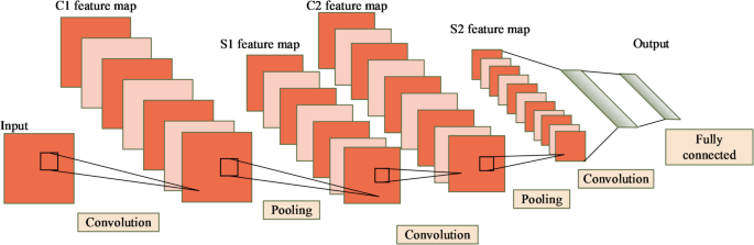
The 2D-CNNs are an important model in deep learning for processing image data. It extracts spatial features through local connections and weight sharing³². The 2D-CNNs consist of several layers: the input layer, convolutional layers, pooling layers, and fully connected layers. The core operation of the 2D-CNNs is the convolution operation. The architecture of the 2D-CNNs are shown in Fig. 1.

2D-CNNs structure.

For an input image \(\:X\in\:{\mathbb{R}}^{H\times\:W\times\:C}\), where \(\:H\) and \(\:W\) represent the height and width of the image, and \(\:C\) represents the number of channels. The output feature map from the convolutional layer, \(\:Y\in\:{\mathbb{R}}^{{H}^{{\prime\:}}\times\:{W}^{{\prime\:}}\times\:K}\), can be computed using the Eq. (10):

\(\:{W}_{p,q,c,k}\) is the weight of the convolutional kernel (filter), with dimensions \(\:P\times\:Q\times\:C\times\:K\), where \(\:P\) and \(\:Q\) are the height and width of the kernel, respectively, and \(\:K\) is the number of kernels. \(\:{b}_{k}\) is the bias term, and σ(⋅) is the activation function, typically using the “Rectified Linear Unit (ReLU)” function: \(\:\sigma\:\left(x\right)=\text{m}\text{a}\text{x}(0,x)\).

The convolution process is shown in Fig. 2.

Convolution process.

Pooling operations are typically used to reduce the dimensionality of the feature map, thereby decreasing the computational load and mitigating overfitting. In 2D image tasks, the target object does not always appear in a fixed position but can appear at some offset from its initial position. To alleviate the positional sensitivity of the convolution layer, pooling operations were introduced³³. Additionally, pooling operations can significantly reduce the number of parameters and eliminate redundant information, without affecting the image’s information expression. Common pooling methods include Max Pooling and Mean Pooling. Max Pooling selects the maximum value within the pooling window, which helps preserve edge details, while Mean Pooling computes the average value within the window, emphasizing background information. Diagrams of both pooling computations are shown in Fig. 3.

Diagrams of two pooling computations.

In Fig. 3, for an image of size 4 × 4, a sliding pooling window of size 2 × 2 is used with a stride of 2. This means that after sliding 2 steps, the maximum value within the pooling window is taken as the output for Max Pooling; for Mean Pooling, the average value within the window is taken as the output.

Assuming the pooling kernel is R×S, the pooled output \(\:Z\in\:{\mathbb{R}}^{{H}^{{\prime\:}{\prime\:}}\times\:{W}^{{\prime\:}{\prime\:}}\times\:K}\) can be defined using the Equation (for Max Pooling as an example):

The fully connected layer is used to map the extracted features to the target output space³⁴. Suppose the features output by the pooling layer are flattened into a vector \(\:\text{z}\in\:{\mathbb{R}}^{d}\), then the output of the fully connected layer \(\:\mathbf{o}\in\:{\mathbb{R}}^{n}\) can be calculated using the Eq. (12):

In the optimization process, the 2D-CNNs update the network parameters through the backpropagation algorithm to minimize the loss function L. For example, the cross-entropy loss is calculated as shown in Eq. (13):

\(\:N\) is the number of samples; \(\:M\) is the number of classes; \(\:{y}_{i,j}\) is the true label; \(\:{\widehat{y}}_{i,j}\) is the predicted probability distribution by the model³⁵. Through multilayer stacking and parameter optimization, 2D-CNNs can effectively extract spatial features in learning behavior pattern recognition tasks, achieving efficient classification and prediction.

3D-CNNs

The 3D-CNNs are an important model in deep learning for processing spatiotemporal information, especially for feature extraction from video or three-dimensional volumetric data^36,37. A diagram of 3D convolution is shown in Fig. 4.

Diagram of 3D convolution.

For the input data \(\:X\in\:{\mathbb{R}}^{T\times\:H\times\:W\times\:C}\), where \(\:T\) represents the temporal dimension, \(\:H\) and \(\:W\) are the height and width of the image, and \(\:C\) is the number of channels, the output feature map of the 3D convolution operation \(\:{Y\in\:\mathbb{R}}^{{T}^{{\prime\:}}\times\:{H}^{{\prime\:}}\times\:{W}^{{\prime\:}}\times\:K}\) can be computed using the following Eq. (14):

\(\:{W}_{r,p,q,c,k}\) is the weight of the 3D convolution kernel, with size \(\:R\times\:P\times\:Q\times\:C\times\:K\), where \(\:R\) represents the temporal dimension of the convolution kernel³⁸.

Similar to 2D-CNN, the 3D-CNNs also include pooling layers to reduce the dimensionality of the feature maps, but the pooling operation is extended to the temporal dimension. Assuming the pooling kernel size is \(\:{S}_{T}\times\:{S}_{H}\times\:{S}_{W}\), the pooled output \(\:Z\in\:{\mathbb{R}}^{{T}^{{\prime\:}{\prime\:}}\times\:{H}^{{\prime\:}{\prime\:}}\times\:{W}^{{\prime\:}{\prime\:}}\times\:K}\) can be defined by Eq. (15):

The 3D-CNNs can extract temporal features for behavior pattern analysis³⁹. For example, in behavior recognition, motion changes between frames are key features, and 3D convolution jointly models spatial and temporal features by stacking temporal information.

Quantum convolutional neural network

The hybrid Quantum Convolutional Neural Network (QCNN) mainly consists of key components such as the quantum convolutional layer, pooling layers, and fully connected layers. In this architecture, the quantum convolutional layer uses quantum convolutional kernels instead of traditional classical convolutional kernels. It leverages the high concurrency and exponential storage capacity of quantum computing. This approach accelerates the convolution process⁴⁰. The pooling layer combines classical and quantum computing, introducing three types of pooling methods: Max Pool, Avg Pool, and Quantum Pool, to accommodate the quantum convolutional kernels and efficiently and accurately extract features⁴¹. The fully connected layer, implemented via a classical feedforward neural network, is used to complete the action recognition task. The formalization of the hybrid QCNN is shown in (16):

\(\:{U}_{i}\left(\theta\:\right)\) represents the quantum convolutional layer, \(\:{U}_{0}\left(\text{x}\right)\) represents quantum state encoding, \(\:{P}_{i}\left(\theta\:\right)\) represents the pooling layer, and \(\:{F}_{i}\left(\theta\:\right)\) represents the classical fully connected layer. The quantum convolutional layer is primarily composed of quantum convolutional kernels⁴². These kernels are constructed using low-depth, strong entanglement, and lightweight parameterized quantum circuits. The quantum circuits utilize two qubits and perform complex convolutional tasks through a one-dimensional convolution approach. The quantum convolutional kernel is formed by sequentially arranging quantum convolutional blocks (QCB), which enhances its expressiveness and scalability. The quantum convolutional layer replaces the classical computational methods with quantum computing, fully exploiting quantum entanglement and parallelism. It retains the two key features of classical CNNs: local connectivity and weight sharing. This not only reduces the complexity of the network model but also significantly improves the computational efficiency of the model⁴³.

The pooling layer enhances the prominent features of the data through downsampling operations, achieving dimensionality reduction and, to some extent, reducing the risk of network overfitting.

The fully connected layer is implemented through a classical feedforward neural network in machine learning. It uses the features extracted by the quantum convolutional layer and pooling layer. These features are then used to predict the output of the classification task. The computation is shown in Eq. (17):

σ(⋅) represents the activation function, \(\:{\theta\:}_{i}^{T}\) denotes the weight matrix, and b represents the bias parameter. First, the output from the last pooling layer is converted into a one-dimensional vector, which is then used as input for the fully connected layer. Next, this one-dimensional vector is processed by the activation function. The activation function introduces nonlinearity into the vector, thereby completing the task of detecting and identifying malicious code. Additionally, this process also optimizes the model’s training convergence performance.

Data preprocessing

In the study of badminton player motion classification, data preprocessing is a crucial step to ensure the model’s training effectiveness and improve accuracy. The following data preprocessing steps were applied in this study, including data cleaning, feature extraction, data normalization, data augmentation, and data partitioning.

Data collection and cleaning

The raw data used in this study was obtained from video recordings of broadcast and television programs, featuring four different badminton matches. The dataset includes information on athletes’ joint positions, velocities, and accelerations under various stroke techniques. Data cleaning is a crucial initial step. Samples with excessive missing values were removed, and abnormal data points were corrected. Missing data was partially imputed using interpolation methods to ensure data completeness and continuity. Outlier detection was primarily conducted using statistical methods, such as box plots, to identify and eliminate data points that significantly deviated from the mean.

Feature selection

Feature selection is a key step in improving model performance. To better understand the importance of different features in classifying badminton strokes, this study employs a model-based feature selection method to analyze each feature’s contribution to classification accuracy.

Arm angle

The arm angle is a critical feature, particularly in badminton strokes, where the movement pattern and angular variation of the arm directly influence shot accuracy and power. This feature is typically extracted from video frames using human pose estimation techniques, such as OpenPose. By analyzing the relative angular changes between the arm and other body parts, this approach accurately captures the detailed motion of athletes during strokes. In classification tasks, arm angle serves as a key factor in distinguishing different stroke types (e.g., forehand, backhand, and volley). Notably, in the QCNN model, arm angle is identified as the most significant feature, highlighting its essential role in stroke recognition.

Twist angle

The twist angle reflects the degree of upper body rotation during a stroke. In badminton, body rotation—including trunk and upper limb torsion—plays a crucial role in executing serves, forehand, and backhand strokes. The twist angle is typically extracted through pose estimation by analyzing angular changes in the shoulders, elbows, and spine to assess upper body rotation. In the QCNN model, the high significance of the twist angle indicates its importance in differentiating between high-intensity and low-intensity strokes. This feature is particularly indispensable for identifying complex movements, such as backhand volleys.

Footwork position

Footwork position reflects an athlete’s stance and foot movement during a stroke. As a high-intensity and dynamic sport, badminton requires precise footwork for players to reach the optimal hitting position in time. This feature helps determine whether an athlete is positioned correctly for a stroke and aids in distinguishing different shot types. For example, rapid footwork adjustments are often associated with serves or volleys, whereas slower adjustments may correspond to forehand or backhand strokes.

Grip type

it is a key feature closely related to stroke efficiency and execution. It determines the power and angle of a shot, influencing the athlete’s force application mechanism. By analyzing the relative position between the player’s hand and the racket handle, grip type characteristics can be extracted. The significance of this feature lies in the fact that different grips directly affect shot performance. For instance, forehand and backhand strokes require distinct grip techniques, and this variation is crucial for improving the classification performance of the model.

Step length

Step length describes the stride distance an athlete covers when executing a stroke. It reflects agility and explosiveness in movement. This feature is typically extracted using sensors or video-based motion tracking, with stride length calculated based on the time intervals and positional changes between foot placements. In badminton, step length plays a critical role in rapid shot preparation. This is especially true for fast-reaction strokes, such as volleys, where an athlete’s ability to adjust quickly can determine successful execution. Although step length has a relatively lower feature importance score, it still provides valuable supplementary information, helping the model better understand overall movement coordination.

Feature extraction

The goal of this study is to extract useful features from the motion data of athletes. Time-series features were first extracted from the raw data, including joint angles, angular velocity, and acceleration. These features can accurately describe the biomechanical performance of the athlete during different strokes. The specific extraction steps include.

Joint angle calculation

Based on three-dimensional coordinate data, joint angles were computed using the angle formula between vectors. These angles reflect the relative position changes of the athlete’s arm, shoulder, and torso during the stroke.

Angular velocity and acceleration

The angular velocity and acceleration of the joints were obtained by performing time-differencing on the joint angle data, capturing the dynamic features of the athlete’s movements.

Time-domain features

These include the start time and duration of each motion, as basic time-domain information.

Data normalization

To eliminate the influence of varying feature scales, all feature data were normalized. This study used the Z-score normalization method, which zeroes the mean and standardizes the variance of each feature to fit a standard normal distribution. This step ensures that different features have the same importance during training and prevents features with larger ranges from dominating the training process.

The normalization calculation is shown in Eq. (18):

Let X represent the original feature values, μ denote the mean of the feature, and σ represent the standard deviation of the feature.

Data augmentation

To enhance the model’s generalization ability, data augmentation techniques were employed. Due to the diversity and complexity of badminton actions, data augmentation effectively improves the model’s robustness, especially when the dataset is small. The specific augmentation methods used include.

Time shifting

The original data is shifted along the time dimension to simulate variations in the athlete’s actions across different time periods.

Rotation and scaling

Joint position data was subjected to rotation and scaling operations, simulating movements at different angles and postures.

Noise addition

To improve the model’s adaptability to noise, slight Gaussian noise was added to the original data to simulate the imperfections typically found in real-world environments.

Data partitioning

To evaluate the model’s performance, the dataset was divided into training, validation, and test sets. The specific partitioning approach is as follows.

Training set

Used for model training, accounting for 70% of the dataset. The training set includes various types of strokes from the athletes, allowing the model to learn how to distinguish between different action categories.

Validation set

Used to adjust model parameters during training, accounting for 15% of the dataset. The validation set helps to tune hyperparameters such as learning rate, regularization parameters, etc., to optimize model performance.

Test set

Used for final model evaluation, accounting for 15% of the dataset. The test set is not involved in the training process and is used solely to assess the model’s generalization ability and performance.

During the data partitioning process, care was taken to ensure the distribution of each action category remained balanced. This approach helped prevent the model from becoming biased towards certain categories due to class imbalance. Through these steps, the raw data was cleaned, standardized, and augmented, making it suitable for subsequent model training and analysis. These preprocessing operations not only improved the quality of the data but also significantly enhanced the model’s training efficiency and classification accuracy.

Datasets collection and experimental environment

To validate the performance of the proposed method, this study collected data from multiple sources. Specifically, video recordings from broadcast and television programs were utilized, covering four different badminton matches: the 2020 Tokyo Olympics, the 2023 China Masters, the 2023 Sudirman Cup, and the 2023 China Open. These videos were stored in Moving Picture Experts Group Phase 2 (MPEG-2) compression format with a frame size of 352 × 288 pixels. A total of 540 samples were collected, each capturing an athlete’s performance across five different stroke types: serve, forehand, backhand, forehand volley, and backhand volley. Each stroke type was executed 30 times under valid conditions. To ensure consistency, frames were extracted from the MPEG-2 videos using the FFmpeg tool, maintaining a frame rate of 60 fps. Each frame was resized to 352 × 288 pixels to meet the model’s input requirements. Each frame was processed using the OpenPose algorithm for human pose estimation, extracting key joint positions of the athletes, including shoulders, elbows, wrists, waist, knees, and ankles. The annotations consisted of 2D joint coordinates, which were later used for feature computation. The dataset was then split into training (70%), validation (15%), and test (15%) sets. The dataset can be accessed at: https://ai.gitcode.com/datasets?utm_source=highlight_word_gitcode.

The experiments were conducted on a system running Windows 10, with Python 3.8 as the development and execution environment. A GTX 3060 GPU was selected, along with the corresponding Compute Unified Device Architecture (CUDA) version 10.1. This hardware and software configuration effectively supports the TensorFlow 2.1.3 deep learning framework, ensuring computational efficiency and system stability. For interactive development and experiment execution, Jupyter Notebook was used as the primary environment. Video processing tasks, including frame extraction and preprocessing, were performed using OpenCV and FFmpeg libraries.

Parameters setting

Different machine learning and deep learning methods were used, each with its specific hyperparameter settings. Table 1 lists the key parameters used for each method, along with the rationale for their selection.

Performance evaluation

To quantitatively evaluate the algorithm, this study introduces four evaluation metrics: Accuracy (ACC), Precision (P), Recall (R), and F1-score (F1). ACC represents the proportion of correctly predicted samples to the total number of samples. P denotes the proportion of correctly identified positive samples among those predicted as positive. R measures the proportion of actual positive samples that were correctly identified. The F1-score, which is the harmonic mean of precision and recall, provides a comprehensive measure of the model’s performance.

Classification results of different algorithms for various actions

The classification results of different algorithms for various actions are shown in Table 2.

In Table 2, the QCNN model achieved the best performance across all stroke classification tasks, with P, R, F1, and ACC values consistently higher than those of CNN and SVM. For instance, in backhand volley recognition, QCNN achieved an ACC of 0.865, significantly outperforming CNN (0.79) and SVM (0.75). This demonstrates that QCNN exhibits a stronger capability in recognizing complex actions.

The 3D CNN model performed second best in most stroke classifications, surpassing the traditional SVM algorithm. Notably, for serve and backhand strokes, 3D CNN achieved ACC scores of 0.862 and 0.855, respectively, highlighting its advantage in feature extraction and classification. However, in more complex actions such as forehand volley and backhand volley, 3D CNN still has room for improvement. SVM showed stable performance in recognizing simpler actions (e.g., serve and forehand strokes). However, its performance dropped significantly in complex actions such as volleys. For example, in forehand and backhand volleys, SVM achieved ACC scores of 0.735 and 0.75, respectively, which were substantially lower than those of QCNN and 3D CNN. This indicates that SVM struggles with high-dimensional and complex spatiotemporal features, whereas QCNN and 3D CNN are better suited for such tasks.

The confusion matrices of all models are shown in Fig. 5.

Confusion matrices of different models.

Figure 5 provides an intuitive representation of each model’s classification accuracy for different stroke types, as well as their misclassification patterns. The analysis is as follows.

• SVM Confusion Matrix: In the classification of serves and forehand strokes, the diagonal values are relatively high, indicating that SVM has a certain ability to recognize these simple movements. However, some misclassifications still occur. In contrast, for forehand and backhand volleys, the non-diagonal elements increase significantly, meaning that forehand volleys may be misclassified as backhand volleys and vice versa. This highlights SVM’s limitations in handling complex strokes, making it difficult to precisely distinguish between different movement categories.

• 3D CNN Confusion Matrix: Compared to SVM, 3D CNN shows higher proportions of diagonal elements in the classification of serves and backhand strokes, suggesting improved recognition accuracy for these strokes and better feature extraction capabilities. However, when classifying forehand and backhand volleys, while the number of misclassifications is lower than that of SVM, some non-diagonal elements remain. This indicates that despite the model’s advantages in processing spatiotemporal features, there is still room for improvement in distinguishing complex strokes.

• QCNN Confusion Matrix: QCNN achieves the highest proportion of diagonal elements across all stroke types, demonstrating superior classification accuracy. For complex strokes such as forehand and backhand volleys, QCNN shows minimal misclassification, with significantly lower non-diagonal values. This highlights QCNN’s remarkable capability in capturing spatiotemporal features, making it highly effective at differentiating between various stroke types.

Model robustness and noise resistance analysis

To evaluate the robustness and noise resistance of different models, noise processing was introduced into both the training and test datasets, and the classification accuracy of various algorithms was compared under noisy conditions. Noise was introduced by adding Gaussian noise to the original data, simulating potential errors or inaccuracies that may arise during an athlete’s movement. The models—SVM, 3D CNN, and QCNN—were tested under different noise intensities: low, medium, and high noise levels.

The specific noise configurations were as follows:

• Low Noise (0.1): Gaussian noise with a mean of 0 and a standard deviation of 0.1 was added to the input data to simulate minor data collection errors, such as small fluctuations in sensor readings or slight tremors under normal conditions.

• Medium Noise (0.3): Gaussian noise with a standard deviation of 0.3 was applied to simulate moderate data inaccuracies, such as slight inconsistencies in hand or body movements and measurement deviations caused by varying angles of the recording equipment.

• High Noise (0.5): Gaussian noise with a standard deviation of 0.5 was introduced to simulate extreme noise conditions, such as sensor jitter caused by high-speed movements, occlusions, or environmental light interference, which challenge a model’s noise resistance.

This study employs torch.randn_like(image) * noise_level to generate random Gaussian noise, which is then added to the original data. This approach allows for the evaluation of the classification accuracy of different algorithms (SVM, CNN, and QCNN) under various noise conditions, thereby validating their robustness and noise resistance. The specific results of the model robustness and noise resistance analysis are presented in Table 3.

The results indicate that QCNN exhibits significant robustness advantages across all noise levels. Under low-noise conditions, QCNN achieves an ACC of 0.945, notably higher than 3D CNN’s 0.915 and SVM’s 0.902. As noise levels increase, QCNN maintains an ACC of 0.913 under medium noise, while 3D CNN and SVM experience performance drops to 0.862 and 0.818, respectively. Even under high-noise conditions, QCNN sustains an ACC of 0.882, whereas 3D CNN and SVM further decline to 0.78 and 0.715, respectively. These findings demonstrate QCNN’s superior resistance to noise, enabling it to maintain high classification accuracy despite data contamination.

In contrast, SVM and 3D CNN exhibit a pronounced decline in performance as noise levels increase. SVM achieves only 0.715 ACC under high noise, revealing its limitations in complex noisy environments. While 3D CNN performs reasonably well under low-noise conditions, its accuracy drops to 0.78 at high noise levels, indicating limited adaptability to noise. Overall, QCNN’s robustness makes it more suitable for real-world applications where noise interference is a concern.

Feature selection and importance analysis

A decision tree-based feature importance scoring method was employed to evaluate the features extracted by SVM, 3D CNN, and QCNN. The results reveal that, across all three models, the most critical features are athlete posture, racket-swing motion, and footwork variations. In particular, QCNN assigns high importance scores to posture-related features, especially arm angles, and racket-swing motion, indicating their strong contribution to model performance. The feature importance scores for each action type, along with their rankings across different algorithms, are presented in Table 4.

In Table 4, arm angle and rotation angle have the most significant impact on action classification. Notably, in QCNN, the arm angle feature received the highest importance score, indicating that the model effectively leverages spatiotemporal features to distinguish different types of strokes. In contrast, the feature importance distribution in SVM and 3D CNN is more balanced, but these models exhibit relatively weaker performance in differentiating swing speed and footwork position.

To evaluate the impact of optimized feature selection on model performance, the QCNN model was trained using both the full feature set and an optimized feature set. The accuracy and F1-score on the test set were recorded, and the performance evaluation results before and after feature selection optimization are shown in Fig. 6.

Performance evaluation of the model before and after feature selection optimization.

Further analysis indicates that optimizing feature selection can effectively enhance model classification performance. After feature filtering, the QCNN model was trained using arm angle, rotation angle, and swing speed as the primary input features. With the optimized feature set, the accuracy and F1-score of the QCNN model improved by approximately 5% and 4%, respectively. This demonstrates that optimizing feature selection can significantly enhance classification performance. Compared to the 2D-CNN proposed by Van Herbruggen et al. (2024)⁴⁴, the accuracy of the QCNN model improved from 0.909 to 0.945. Additionally, when compared to the LSTM framework introduced by Malik and Jain (2023)⁴⁵, the F1-score of QCNN increased from 0.84 to 0.947. These comparative results further validate the superiority of the QCNN model.

Complexity analysis of classifiers

In order to comprehensively evaluate the performance of classifiers such as SVM, 3D CNN, and QCNN, this study analyzes their complexity from the perspectives of training time and inference time. The experimental results are shown in Table 5.

Table 5 shows that SVM has a training time of 120 s and an inference time of 0.01 s, demonstrating high efficiency and suitable for processing simple or moderately complex data. In contrast, the training time of 3D CNN is significantly longer, reaching 3600 s, but its inference time is still relatively fast, at 0.1 s. This indicates that although 3D CNN has high computational complexity when processing spatiotemporal data, it can still maintain a certain level of real-time performance. However, QCNN has the longest training time of 4200 s and the longest inference time of 0.2 s, which reflects the high computational cost of quantum computing in processing complex data. Nevertheless, QCNN has higher accuracy and robustness in processing complex pattern recognition tasks, making it suitable for applications that require high precision.

Performance comparison with other motion recognition models

To comprehensively evaluate the performance of the proposed QCNN-based badminton player motion detection technology, its experimental results are compared with five other machine learning based motion recognition models. These models include: RF, KNN, DT, LSTM, and SACNN. The comparison results are shown in Fig. 7.

Performance comparison with other motion recognition models.

The data in Fig. 7 suggests that QCNN outperforms the other five motion recognition models in performance indicators such as accuracy, precision, recall, and F1 score. Specifically, the accuracy of QCNN reaches 0.965, significantly higher than LSTM (0.830), SACNN (0.875), RF (0.820), KNN (0.780), and DT (0.750). Its accuracy (0.972), recall (0.968), and F1 score (0.965) are also higher than other models, indicating that QCNN has higher classification accuracy and robustness in identifying different hitting actions of badminton players. In contrast, traditional machine learning models such as RF, KNN, and DT perform poorly in handling complex motion data, while deep learning-based LSTM and SACNN, although performing well, still cannot compete with QCNN.

Discussion

In this study, the performance of different algorithms in the classification of badminton player movements is analyzed. The experimental results indicate that, the QCNN model exhibits the highest accuracy among all categories of hitting styles, especially in dealing with complex spatiotemporal features. Although traditional machine learning algorithms such as SVM and 2D CNN can also achieve excellent results, 3D CNN and QCNN models perform more prominently when dealing with complex time series data. The feature selection process indicates that dynamic features such as joint angles and angular velocities play a crucial role in action recognition. In feature importance analysis, shoulder angle has a significant impact on forehand stroke classification. Although the model performs well, noise and environmental factors may affect motion capture data, and future research can further explore how to improve the robustness of the model.

This study has the following novelty and advantages: (1) Novelty: For the first time, QCNN is applied to the field of badminton athlete motion detection, providing new ideas and methods for motion detection technology. (2) Advantage: QCNN has significant advantages in classification performance, with higher accuracy, recall, and F1 score than traditional machine learning models and deep learning models. In addition, QCNN has strong adaptability to noisy data and can maintain high classification accuracy in complex environments. However, this study also has some limitations: The training time of QCNN is longer and requires more computing resources. In addition, quantum computing technology is still in the development stage, and the limitations of its hardware and software environment may affect the widespread application of the model. Future research could further optimize the training algorithm of QCNN, improve its training efficiency, and explore its applications in other sports fields.

Research contribution

The QCNN model used here performs well in badminton athlete motion detection, with an accuracy of 96.5%, significantly better than traditional machine learning models and deep learning models. This indicates that QCNN has stronger classification ability and robustness when processing complex motion data. Additionally, QCNN has strong adaptability to noisy data and can maintain high classification accuracy in complex environments. Therefore, QCNN provides an effective method for detecting the movement of badminton players. The main contributions of this study include: applying QCNN to badminton action classification and demonstrating their advantages in complex pattern recognition; deeply exploring the process of extracting motion features and identifying dynamic and static features that are crucial for classification tasks; Algorithm comparison and evaluation: making a detailed comparison of SVM, 2D CNN, 3D CNN, QCNN and other algorithms, demonstrating the advantages and disadvantages of each algorithm in action recognition.

Future works and research limitations

This study does have certain limitations, and future research can be improved in the following areas: (1) Noise Handling: Future research could explore better ways to handle environmental noise, enhancing the model’s robustness. (2) Cross-Sport Application: This method can be extended to other sports, such as tennis or table tennis. Future research could explore the cross-domain adaptability of the model. (3) Real-Time Application: The current model is based on pre-collected data. In the future, the algorithm could be optimized to enable real-time classification during training or competition. (4) Further Applications of Quantum Computing: As quantum computing progresses, more advanced quantum algorithms could be incorporated into QCNN to improve training efficiency and classification accuracy. In conclusion, while this study has made significant contributions to badminton action recognition, there is still much room for improvement. Future research can continue to explore these directions.

Authors and Affiliations

1. School of Physical Education, Fujian Polytechnic Normal University, Fuzhou, 350300, China

   Xuanmin Zhu

2. Faculty of Education, Silpakorn University, Sanam Chandra Palace Campus, Amphoe Muang, Nakhon Pathom, 73000, Thailand

   Lizhi Liu, Jingshuo Huang & Xi Ling

3. Chengyi University College, Jimei University, Xiamen, 361021, China

   Genyan Chen

4. Science of Physical Education, Fujian Normal University, Fuzhou, 350117, China

   Yanshuo Chen

Contributions

Xuanmin Zhu: Conceptualization, methodology, software, validation, formal analysis, investigation, resources, data curation, writing—original draft preparationLizhi Liu: methodology, software, validation, formal analysisJingshuo Huang: validation, formal analysis, investigation Genyan Chen: resources, data curationXi Ling: writing—review and editing, visualization, supervision, project administration, funding acquisitionYanshuo Chen: visualization, supervision.

Corresponding author

Correspondence to Xi Ling.

Competing interests

The authors declare no competing interests.

Ethical approval

The studies involving human participants were reviewed and approved by Faculty of Education, Silpakorn University Ethics Committee (Approval Number: 2022.0214200). The participants provided their written informed consent to participate in this study. All methods were performed in accordance with relevant guidelines and regulations.

Publisher’s note

Springer Nature remains neutral with regard to jurisdictional claims in published maps and institutional affiliations.

Open Access This article is licensed under a Creative Commons Attribution-NonCommercial-NoDerivatives 4.0 International License, which permits any non-commercial use, sharing, distribution and reproduction in any medium or format, as long as you give appropriate credit to the original author(s) and the source, provide a link to the Creative Commons licence, and indicate if you modified the licensed material. You do not have permission under this licence to share adapted material derived from this article or parts of it. The images or other third party material in this article are included in the article’s Creative Commons licence, unless indicated otherwise in a credit line to the material. If material is not included in the article’s Creative Commons licence and your intended use is not permitted by statutory regulation or exceeds the permitted use, you will need to obtain permission directly from the copyright holder. To view a copy of this licence, visit http://creativecommons.org/licenses/by-nc-nd/4.0/.

Reprints and permissions

References

Luo, J. et al. Vision-based movement recognition reveals badminton player footwork using deep learning and binocular positioning. Heliyon 8 (8), 7–12 (2022).
De Waelle, S. et al. The use of contextual information for anticipation of badminton shots in different expertise levels. Res. Q. Exerc. Sport. 94 (1), 15–23 (2023).
Lin, K. C. et al. The effect of real-time pose recognition on badminton learning performance. Interact. Learn. Environ. 31 (8), 4772–4786 (2023).
Dasgupta, A. et al. Machine learning for optical motion capture-driven musculoskeletal modelling from inertial motion capture data. Bioengineering 10 (5), 510 (2023).
Alsaif, K. I. & Abdullah, A. S. Computer vision systems and deep learning for the recognition of athlete’s movement: A review Article. Tikrit J. Pure Sci. 28 (6), 180–191 (2023).
Abdullah, A. S. & AlSaif, K. I. Computer vision system for backflip motion recognition in gymnastics based on deep learning. J. Al-Qadisiyah Comput. Sci. Math. 15 (1), 150–157 (2023).
Kranzinger, C. et al. Classification of human motion data based on inertial measurement units in sports: A social review. Appl. Sci. 13 (15), 8684 (2023).
Dorschky, E. et al. Perspective on in the wild movement analysis using machine learning. Hum. Mov. Sci. 87 (2), 103042 (2023).
Wahab, H. et al. Machine learning based small bowel video capsule endoscopy analysis: challenges and opportunities. Future Generation Comput. Syst. 143 (6), 191–214 (2023).
Slemenšek, J. et al. Human gait activity recognition machine learning methods. Sensors 23 (2), 745 (2023).
Hu, Z. et al. Machine learning for tactile perception: advancements, challenges, and opportunities. Adv. Intell. Syst. 5 (7), 2200371 (2023).
Ooi, J. H. & Gouwanda, D. Badminton stroke identification using wireless inertial sensor and neural network. Proc. Inst. Mech. Eng. P J. Sports Eng. Technol. 237 (4), 291–300 (2023).
Liu, J. & Liang, B. An action recognition technology for badminton players using deep learning. Mob. Inform. Syst. 2022 (1), 3413584 (2022).
Deng, J., Zhang, S. & Ma, J. Self-attention-based deep Convolution LSTM framework for sensor-based badminton activity recognition. Sensors 23 (20), 8373 (2023).
Zheng, Y. & Liu, S. Bibliometric analysis for talent identification by the subject–author–citation three-dimensional evaluation model in the discipline of physical education. Libr. Hi Tech. https://doi.org/10.1108/LHT-12-2019-0248 (2020).
Asriani, F., Azhari, A. & Wahyono, W. Improving badminton action recognition using 11:23 2025/1/27spatio-temporal analysis and a weighted ensemble learning model. Computers Mater. Continua. 81 (2), 156 (2024).
Pu, Y., Gao, X. & Lv, W. Design of optical tracking sensor based on image feature extraction for badminton athlete motion recognition. Opt. Quant. Electron. 56 (4), 608 (2024).
Zhang, T. Application of optical motion capture based on multimodal sensors in badminton player motion recognition system. Opt. Quant. Electron. 56 (2), 275 (2024).
Seong, M. et al. MultiSenseBadminton: wearable sensor–based Biomechanical dataset for evaluation of badminton performance. Sci. Data. 11 (1), 343 (2024).
Wang, B. et al. Recognition of semg hand actions based on cloud adaptive quantum chaos ions motion algorithm optimized Svm. J. Mech. Med. Biology. 19 (06), 1950047 (2019).
Ou, H. & Sun, J. Multi-scale Spatialtemporal information deep fusion network with Temporal pyramid mechanism for video action recognition. J. Intell. Fuzzy Syst. 41 (3), 4533–4545 (2021).
Malibari, A. A. et al. Quantum water Strider algorithm with hybrid-deep-learning-based activity recognition for human–computer interaction. Appl. Sci. 12 (14), 6848 (2022).
Yao, L. et al. Action unit classification for facial expression recognition using active learning and SVM. Multimedia Tools Appl. 80 (2), 24287–24301 (2021).
Abdullah, D. M. & Abdulazeez, A. M. Machine learning applications based on SVM classification a review. Qubahan Acad. J. 1 (2), 81–90 (2021).
Patel, C. I. et al. Histogram of oriented gradient-based fusion of features for human action recognition in action video sequences. Sensors 20 (24), 7299 (2020).
Abdelbaky, A. & Aly, S. Two-stream Spatiotemporal feature fusion for human action recognition. Visual Comput. 37 (7), 1821–1835 (2021).
Ahad, M. A. R. et al. Action recognition using kinematics posture feature on 3D skeleton joint locations. Pattern Recognit. Lett. 145 (4), 216–224 (2021).
Pareek, P. & Thakkar, A. A survey on video-based human action recognition: recent updates, datasets, challenges, and applications. Artif. Intell. Rev. 54 (3), 2259–2322 (2021).
Sun, Z. et al. Human action recognition from various data modalities: A review. IEEE Trans. Pattern Anal. Mach. Intell. 45 (3), 3200–3225 (2022).
Li, C. et al. Surface EMG data aggregation processing for intelligent prosthetic action recognition. Neural Comput. Appl. 32 (2), 16795–16806 (2020).
Wang, Z. et al. Research on human behavior recognition in factory environment based on 3-2DCNN-BIGRU fusion network. Signal. Image Video Process. 19 (1), 1–12 (2025).
Ullah, H. & Munir, A. Human action representation learning using an attention-driven residual 3dcnn network. Algorithms 16 (8), 369 (2023).
Hussain, A. et al. Shots segmentation-based optimized dual-stream framework for robust human activity recognition in surveillance video. Alexandria Eng. J. 91, 632–647 (2024).
Habib, S. et al. Abnormal activity recognition from surveillance videos using convolutional neural network. Sensors 21 (24), 8291 (2021).
Toraman, S. Preictal and interictal recognition for epileptic seizure prediction using pre-trained 2DCNN models. Traitement Du Signal. 37 (6), 524 (2020).
Vrskova, R. et al. Human activity classification using the 3DCNN architecture. Appl. Sci. 12 (2), 931 (2022).
Yao, G., Lei, T. & Zhong, J. A review of convolutional-neural-network-based action recognition. Pattern Recogn. Lett. 118 (3), 14–22 (2019).
Le, T. H., Le, T. M. & Nguyen, T. A. Action identification with fusion of BERT and 3DCNN for smart home systems. Internet Things. 22 (1), 100811 (2023).
Dhiman, C., Vishwakarma, D. K. & Agarwal, P. Part-wise spatio-temporal attention driven CNN-based 3D human action recognition. ACM Trans. Multimidia Comput. Commun. Appl. 17 (3), 1–24 (2021).
Sathya, T. & Sudha, S. OQCNN: optimal quantum convolutional neural network for classification of facial expression. Neural Comput. Appl. 35 (12), 9017–9033 (2023).
Kawakura, S. & Shibasaki, R. Quantum neural network-based deep learning system to classify physical timeline acceleration data of agricultural workers. Eur. J. Agric. Food Sci. 2 (6), 23–26 (2020).
Amin, J. et al. Detection of anomaly in surveillance videos using quantum convolutional neural networks. Image Vis. Comput. 135 (3), 104710 (2023).
Das, S., Martina, S. & Caruso, F. The role of data embedding in equivariant quantum convolutional neural networks. Quantum Mach. Intell. 6 (2), 82 (2024).
Van Herbruggen, B. et al. Strategy analysis of badminton players using deep learning from IMU and UWB wearables. Internet Things. 27 (1), 101260 (2024).
Malik, A. & Jain, R. Badminton action analysis using LSTM. In 2023 International Conference on Applied Intelligence and Sustainable Computing (ICAISC), vol. 1, 1–6 (IEEE, 2023).
Ethics declarations