通过基于操作员的双极复杂模糊语言多属性决策技术来选择用于预测残疾疾病的AI模型

人工智能模型的残疾疾病预测可以描述为旨在以高精度处理医疗数据和查找疾病标记的精心算法。这些复杂的算法系统使用大量医学数据，例如患者病史，遗传信息，临床评估，成像研究和生理监测，以得出与残疾相关疾病的预后。在使用基于AI的诊断模型的同时，可以一次分析多个参数，并且该算法将能够识别不太明显的人眼的连接。这些模型对于由神经，遗传和环境因素决定的残疾疾病特别有用。他们可以结合一个个体数据流，例如神经影像学扫描，遗传测序数据，症状的患者日记以及患者的长期健康记录，以发展高水平的预后模型。这些模型使用多种形式的人工智能，例如深神经网络，支持向量机，决策树和集合学习算法，用于许多机器学习任务，包括疾病表现的可能性，疾病进展率以及可能的治疗方法。这种AI模型的基本目的不仅是诊断工具本身，而且还使用诊断数据来构建可能能够逮捕或可能包含适当医疗干预的疾病的预警系统。

选择适当的AI模型来预测残疾疾病的决策过程被证明是MCDA问题的经典示例，因为其复杂性和决策过程中涉及的多个标准。那些参与医疗保健技术领域决策过程的人在没有一个因素可以用于评估AI模型的适当性的环境中工作。MCDM方法非常关键，因为它可以立即对几种，有时是竞争的标准进行集成评估。当应用于残疾疾病预测时，决策专家面临着几个矛盾的目标，例如预测准确性，计算成本，模型解释性和不同人群的可转移性。传统的决策模型不足以解决问题，因为它们不允许正确考虑这些多个属性及其权衡。AI模型可能具有很高的可预测性，但是它可能会消耗大量的计算能力，或者可能非常可解释但准确。MCDM框架提供了一种系统的方法，可以以定量和定性的方式来衡量这些竞争维度，以便决策者可以开发出比单纯的线性权衡更复杂的有效评分系统。例如，使用AHP，TOPSIS或WAWPA，医疗保健技术专家可以创建一种合理，合理且不可挑选的方法来选择正确的AI模型。这种方法认识到选择不是要寻找理想模型，而是寻找在残疾疾病背景下提供几种重要绩效指标的最佳解决方案。

随着世界的发展和随着时间的流逝，信息或数据变得越来越复杂。因此，酥脆集的概念不足以处理如此棘手和尴尬的信息或数据，因此，Zadeh¹描述了模糊集（FS）理论。FS的每个元素都有会员学位（MD）\（0 \）和\（1 \）， 包括\（0 \）和\（1 \）。之后，许多学者在各个学科中都采用了FS。FS证明了对基于人类知识的鼓励和有力的贡献，可以在多个部门（例如图像编码，数据分析，智能系统等）中取得进步。FS可以通过协作成功地管理多种真正的生活问题，这可能已经超过了传统方法的能力。因此，FS可以处理许多问题，例如DM，处理信息，优化，模式识别等。²解释了模糊顺序（FO）等效类。Xiao等人研究了基于模糊关系（FR）不平等的服务器到客户层架构中的分类。³。Behzadipour等。⁴设计了FS中的层次动态组决策方法。Raiabpour等⁵启动模糊的AHP和Dematel，用于2型模糊，Saranya和Saravanan⁶被诊断出模糊的剧烈和模糊剧烈l。Gitinavard等。⁷在犹豫的FS和Gitinavard和Zarandi中设计了一种排名和平衡的方法⁸用犹豫的FS讨论了软计算方法。Borujeni等。⁹在直觉FS中设计了小组决策分析。Gitinavard和Zarandi解释了混合专家评估方法和间隔价值犹豫FS的小组优势技术¹⁰和Gitinavard等。¹¹分别。各种学者概括的FS和双极模糊（BF）集（BFS）的概念是张诊断的FS的概括之一¹²为了克服FS结构中所呈现的缺乏，即负面方面。BF集的每个元素在\（0 \）和1，包括\（0 \）和1以及负面会员学位（NMD）\（-1 \）和\（0 \）， 包括\（-1 \）和\（0 \）。BF集由多种学者（例如Poulik和Ghorai）使用¹³启动图完整学位，akram¹⁴定义的BF图及其应用，Rajeshwari等。¹⁵Lu等人的拓扑指数的启动BF图。¹⁶BF入射图的诊断循环连通性指数，Sarwar和Akram等。¹⁷探索了BF竞争图。辛格¹⁸使用基于颗粒的加权熵来解释BF概念的减少。Abughazalah等。¹⁹通过使用BF集，描述了BCI代数中的某些理想。Alghamdi等。²⁰启动BF BCK子模型。对于BF集，许多学者定义了各种方法，例如Garai等人。²¹和Alghamdi等。²²定义的多标准DM（MCDM），Zhao等。²³启动了CPT-TODIM方法，Akram和Arshad²⁴定义的Topsis和Electric-I，Akram和Al-Kenani²⁵定义的electre-ii。此外，某些研究人员还研究了Riaz等人等BF集的AO。²⁶启动三角AOS和Jana等。^{27，，，，28}探索了Dombi并优先考虑AOS。Zararsiz和Riaz²⁹开发的BF度量空间。Jamil和Riaz³⁰对于立方BF组启动了TPOSID和Eleptre-I。

FS的另一个概括是Ramot等人研究的复杂模糊（CF）集。³¹为了克服缺陷，在FS的结构（即第二维（额外的模糊信息））中提出。CF集的每个元素都在复杂平面的单位圆圈内具有MD。Tamir等。³²还检查了CF集合，并考虑了每个MD的复杂计划中的单元正方形。在Ramot等人定义的概念中，MD是极性形式的。³¹在Tamir等人的概念中以笛卡尔形式的形状。³²。辛格³³研究了使用香农熵的清晰产生的CF概念分析。Hu等。³⁴CF操作的同质性。可汗等人。³⁵在CF设置下研究了信号处理。Bi等。^{36，，，，37}提出的算术和几何AOS。之后，Mahmood和Rehman³⁸进一步概括了FS概念，并构建了双极复杂的模糊（BCF）集（BCFS），以克服缺陷，该缺陷在FS结构（即第二维（额外的模糊信息）和信息的负面方面）中呈现。BCF集的每个元素都在单位正方形的第一个象限内以及在复合平面的单位正方形的第三象限内都具有PMD。Rehman和Mahmood³⁹描述了BCF集的广义骰子相似性度量（SMS）。Mahmood等。⁴⁰在BCF设置下引入了AO。Ur Rehman等。⁴¹在Frank AOS下引入了BCF设置的分析层次结构过程。Mahmood等。⁴²BCF集的定义的Bonferroni平均操作员。Mahmood和Rehman研究了BCF组的Dombi和Hamacher AOS⁴³和Mahmood等。⁴⁴分别。Mahmood等人引入了BCF软集的概念。⁴⁵。

动机和研究问题

当前选择用于残疾疾病预测的AI模型的方法缺乏足够的解决方案来处理在决策过程中出现的多种不确定性。这项研究研究了一个基本问题，如下

`通过同时解决不确定性，双极性，额外的模糊信息和语言不重点，如何通过同时解决不确定性，双极性，如何增强残疾疾病预测的准确性？

在当前选择用于预测残疾疾病的AI模型的方法中，一个主要差距是，决策（DM）过程涉及各种不确定性和双极性，例如Kumar等人。⁴⁶设计了一个用于疾病预测的MCDM⁴⁷林等人设计的用于预测和诊断精神残疾的多标准技术。⁴⁸讨论了预测疾病状况的机器学习方法，Kumar等人。⁴⁹设计了一种MCDM疾病预测方法。在模型选择方面，这些未解决的方面构成了一个大问题。在许多情况下，选择过程中涉及的属性模棱两可，具有双极性质，可能包含额外的信息，并使用现有选择方法中未完全解决的语言术语。先前选择用于残疾疾病预测模型的策略主要是常规的，并且不能充分纳入DM过程。当前的AI模型选择过程取决于确定性方法，没有足够能力处理复杂性的能力，包括属性模糊度量测量双极评估标准以及额外的模糊信息和语言术语。缺乏这些基本维度会导致选择可预测残疾疾病的AI模型的方法。当前的决策方法显示出固有的局限性，因为它们错过了良好决策过程所需的基本方面。这项研究开发了一种新的MADM方法，为决策提供了增强的现实框架。新模型采用系统方法来处理模糊的信息，同时集成双极性其他模糊数据和语言术语解释。该方法为模型选择提供了更广泛的战略框架，其中包括上下文意识。本文强调了开发这种先进方法的必要性。当缺乏这种方法时，选择用于预测残疾疾病的AI模型从根本上存在缺陷，并可能次优。这项提出的MADM技术方法为医学研究中的模型选择提供了改进的方法，因为它可以对合适的AI解决方案进行更准确的评估。

此外，由于社会经济环境的越来越困难和人类思想的固有主观性，数值数据可能并不总是足以解决现实生活中DM困境中的模棱两可和不清楚的数据，尤其是在定性因素方面。但是，给出语言变量（LV）形状的评估值要容易得多。因此，扎德⁵⁰描述了语言术语（LTS）集（LTS）的概念。Peng等。⁵¹研究了一个交互式模糊LT集。Wang等。⁵²引入了直觉语言（IL）AOS和Ju等。⁵³基于MSM启动IL AOS。Erol等。⁵⁴研究了犹豫的模糊LT集。Geo等。⁵⁵提出了一个间隔值的双极性不确定语言集。MSM的理论可以探索输入参数之间的相互关系，这是其他AOS的MSM运算符之间的主要区别。MSM的概念是处理DM问题的重要且令人印象深刻的技术。在过去的几年中，MSM在Qin和Liu等FS的情况下引起了很多关注⁵⁶探索了直觉FS（IFS），WEI和LU的MSM AOS⁵⁷此外，已定义的MSM运算符的启动MSM AO仅具有在CRISP，IFS，PFS，ILFS等结构中汇总数据的能力，但在信息或数据中，在BCFL的结构中，在BCFL的结构中是无效的。此外，本文在BCFL框架内开发了新的MADM方法和MSM操作员的扩展。文献中存在多个模糊集的广义框架⁵⁸通过采用额外的会员功能，可以直接建模不确定性。各种学者都促进了嗜嗜嗜性理论，例如阿里和Smarandache⁵⁹解释复杂的嗜嗜性套件和Broumi⁶⁰设计了中性粒细节的概念。我们的研究集中于标准的正面和负面方面以及语言术语，但中性嗜性集仍无法解决标准和语言术语的负面方面，尽管它们具有许多优势。本文使用BCFLS，因为此框架符合实现我们的研究目标所需的要求。

贡献和新颖性

这项研究为MCDM提供了双极复杂的语言麦克洛蛋白对称均值（BCFLMSM）算子，这些均值（BCFLMSM）是选择最佳的残疾疾病预测AI模型的现代解决方案，同时将不确定性与双极性以及其他模糊信息以及其他模糊信息和语言评估一起处理。这项研究具有以下新颖的贡献。

• BCFL中的MSM运营商：本文介绍了四个开创性的操作员，称为双极复杂的模糊语言MSM（BCFLMSM），加权MSM（BCFLWMSM），双MSM（BCFLDMSM）和加权双MSM（BCFLWDMS），这些功能提供了全新的功能，可提供多种二维数字不确定性信息。

• BCFL中决策的理论基础：存在强大的理论结构，证明了这些操作员的必要数学方面，以确保复杂的BCFL实施中可靠，一致的决策过程。

• 新颖的Madm方法论：本文开发了完整的双极复杂模糊语言MADM（BCFL-MADM）技术，该技术整合了四个基本信息处理元素：

  • 通过模糊设置操作处理不确定性

  • 双极性管理通过正和负会员学位

  • 通过复杂数字表示的其他模糊信息

  • 语言术语通过专业的语言变量集成

• 现实世界验证：我们的框架通过将其应用于残疾疾病预测模型选择中，证明了它的卓越性，与传统方法相比，它可以产生卓越的结果。

我们开发的方法通过：高级运营商的数学复杂整合以及对多方面信息的卓越管理，对决策理论有了重大改进，并且该框架为解决挑战性的医疗技术选择问题提供了一个先进的解决方案系统，新方法通过建立一个决策框架来确定当前的医疗AI模型选择实践，以确立一个决策框架，以确定多个信息的多元信息依赖于多种信息，并同时确定。

手稿的布局

在预赛部分，本文解释了BCFL和相关结果的理论。在BCF语言Maclaurin对称平均AO本文的一节在BCFL的设置中扩展了MSM，并解释了诸如BCFLMSM，BCFLWMSM，BCFLDMSM和BCFLWDMSM运算符等聚合BCFLN的AOS。在双极复杂的模糊语言MADM方法``部分，包含一种基于定义的MSM操作员和BCFL设置的MADM方法，然后介绍选择用于预测残疾疾病的AI模型的案例研究。比较分析部分将研究理论与一些当前的理论进行了比较，描述了权力和统治的定义概念。该手稿的结论是在研究中结论 - 部分。

受Mahmood和Ur Rehman提出的BCF概念的启发³³，在这里，我们将最有价值，最有意义的概念（称为BCF语言集（BCFL））一次将元素的PMD和NMD授予某个LT变量。让\（\ Mathcal {H} \）成为通用集，并且\（\ +叠加{\ Mathcal {s}} \）\）成为一组连续的LT\（\ Mathcal {s} = \ left \ {{{\ MathBbm {s}} _ {0}，{\ MathBbm {s}} _ {1}，\ dots，\ dots，\ dots，{\ Mathbm {s}}} _ {。

定义1

⁶¹bcfls\（\ Mathcal {H} \）是结构

在哪里，\（{\ Mathbbm {s}} _ {\ phi \ left（\ mathfrak {h} \ right）} \ in \ intlline {\ Mathcal {s s}}} \），，，，\（{\ Mu} _ {p- \ \ \ \ \ \ \ \ s}} \ left（\ mathfrak {h}} _ {ip- \ Mathcal {z}} \ left（\ Mathfrak {h} \ right）\）\）\）是PMD，\（{\ mu} _ {n- \ Mathcal {z}}} \ left（\ Mathfrak {h}} _ {in- \ Mathcal {z}} \ left（\ Mathfrak {h} \ right）\）\）\）是一个NMD\（{\ mu} _ {rp- \ \ \ m {z}}} \ left（\ Mathfrak {h}和\（{\ Mu} _ {rn- \ Mathcal {z}} \ left（\ Mathfrak {h}，元素\（\ Mathfrak {H} \ in \ Mathcal {H} \）到LT\（{\ Mathbbm {s}} _ {\ phi \ left（\ mathfrak {h} \ right）} \）。集合\（\ Mathcal {z} = \ left（{\ MathBbm {s}} _ {\ phi \ left（\ Mathfrak {\ Mathfrak {h} \ right）}，\ left（{\ Mu} _ {p- \ \ \ \ \ \ \ \ \ \ \ \ {z}}}}} _ {n- \ Mathcal {z}} \ left（\ Mathfrak {h} \ right）\ right）\ right）\ right）= \ left（{\ Mathbbm {s}} _ {\ phi \ phi \ phi \ left（\ phi \ left）} _ {rp- \ Mathcal {z}} \ left（\ Mathfrak {h}} _ {rn- \ Mathcal {z}} \ left（\ Mathfrak {h} \ right）+\ iota {\ mu} _ {\ mu} _ {in- \ mathcal {z}}}}}}}，体现了BCFLN。

定义2

⁶¹BCFLN的得分值（SV）\（\ Mathcal {z} = \ left（{\ Mathbbm {s}} _ {\ phi}，\ left（{\ Mu} _ {p- \ m \ m artercal {z}}}，{\ mu {\ mu} _ {n- \ Mathcal {z}}} \ right）\ right）= \ left（{\ MathBbm {s}} _ {\ phi}，\ left（{\ mu} _ {\ mu} _ {rp- \ nathcal {rp- \ \ \ \ mathcal {z}}}}}+\ \ \ \ \ iota} _ {ip- \ Mathcal {z}}，{\ mu} _ {rn- \ m arncal {z}}}+\ iota {\ mu} _ {in- \ mathcal {z}}}}}}}}}}} \ right）\）\）\）\）\）\）\）\）\）\）被发现为

定义3

⁶¹BCFLN的准确性值（AV）\（\ Mathcal {z} = \ left（{\ Mathbbm {s}} _ {\ phi}，\ left（{\ Mu} _ {p- \ m \ m artercal {z}}}，{\ mu {\ mu} _ {n- \ Mathcal {z}}} \ right）\ right）= \ left（{\ MathBbm {s}} _ {\ phi}，\ left（{\ mu} _ {\ mu} _ {rp- \ nathcal {rp- \ \ \ \ mathcal {z}}}}}+\ \ \ \ \ iota} _ {ip- \ Mathcal {z}}，{\ mu} _ {rn- \ m arncal {z}}}+\ iota {\ mu} _ {in- \ mathcal {z}}}}}}}}}}} \ right）\）\）\）\）\）\）\）\）\）\）被发现为

两个BCFLN之间的比较定律依赖于SV\（s {l} _ {sf} \）和AV\（h {l} _ {af} \）上面发现的下面描述

定理1

\（{\ Mathcal {z}} _ {1} = \ left（{\ MathBbm {s}} _ {{{\ phi} _ {1}}，\ left（{\ mu} _ {\ mu} _ {p - {} _ {n - {\ Mathcal {Z}} _ {1}}} \ right）\ right）= \ left（{\ Mathbbm {s}} _ {{\ phi} _ {\ phi} _ {1} _ {1}}}}}}}，\ left（\ mu} _ {rp - {\ Mathcal {z}} _ {1}}}+\ iota {\ mu} _ {ip - {ip- {\ Mathcal {z}} _ {1}}} _ {1}}，{\ MU} _ {rn - {\ Mathcal {z}} _ {1}}+\ iota {\ mu} _ {in - {in- {\ Mathcal {z}} _ {1}} _ {1}}}}} \ right）\ right）\ right） 和 \（{\ Mathcal {z}} _ {2} = \ left（{\ MathBbm {s}} _ {{{\ phi} _ {2}}}，\ left（{\ mu} _ {\ mu} _ {} _ {n - {\ Mathcal {Z}} _ {2}}} \ right）\ right）= \ left（{\ MathBbm {s}} _ {{\ phi} _ {\ phi} _ {2}}}}}}}}}}，\ left（\ mu {\ mu} _ {rp - {\ Mathcal {z}} _ {2}}+\ iota {\ mu} _ {ip- {ip- {\ Mathcal {z}} _ {2}}} _ {2}}，{\ MU} _ {rn - {\ Mathcal {z}} _ {2}}+\ iota {\ mu} _ {in - {in- {\ Mathcal {z}} _ {2}}}}}}}}} \ right）\ right）\ right）\ \） 是 然后两个BCFLN

1. 1。

   如果\ \（{sl} _ {sf} \ left（{\ Mathcal {z}} _ {1} \ right）<{sl} _ {sf} \ left（{\ Mathcal {Z}} _ {z}} _ {2} _ {2}} \ right）\）\）\）\）\）\）\）， 然后\（{\ Mathcal {Z}} _ {1} <{\ Mathcal {Z}} _ {2} \）;

2. 2。

   如果\（{sl} _ {sf} \ left（{\ Mathcal {z}} _ {1} \ right）> {sl} _ {sf} \ left（{\ MathCal {z}} _ {Z}} _ {2} _ {2}} \ right）\）\）\）\）\）\）\）， 然后\（{\ Mathcal {Z}} _ {1}> {\ Mathcal {Z}} _ {2} \）;

3. 3。

   如果\ \（{sl} _ {sf} \ left（{\ Mathcal {z}} _ {1} \ right）= {sl} _ {sf} \ left（{\ Mathcal {z Z}} _ {Z}} _ {1} _ {1} \ right）\）\）\）\）\）\）\）， 然后

4. 1。

   如果\（{hl} _ {af} \ left（{\ Mathcal {z}} _ {1} \ right）<{hl} _ {af} \ left（{\ Mathcal {Z}}} _ {Z}} _ {2}} _ {2} \ right），\ \），\），\），\）然后\（{\ Mathcal {Z}} _ {1} <{\ Mathcal {Z}} _ {2} \）;

5. 2。

   如果\ \（{hl} _ {af} \ left（{\ Mathcal {z}} _ {1} \ right）> {hl} _ {af} \ left（{\ Mathcal {z}}} _ {Z}} _ {2}} _ {2} \ right），\ \），\），\），\）然后\（{\ Mathcal {Z}} _ {1}> {\ Mathcal {Z}} _ {2} \）;

6. 3。

   如果\ \（{hl} _ {af} \ left（{\ Mathcal {z}} _ {1} \ right）= {hl} _ {af} \ left（{\ Mathcal {Z}}} _ {Z}} _ {2}} _ {2} \ right），\ \），\），\），\）然后\（{\ Mathcal {Z}} _ {1} = {\ Mathcal {Z}} _ {2} \）。

本文的这一部分在BCFL的设置中扩展了MSM，并解释了BCFLNS（例如BCFLMSM，BCFLWMSM，BCFLDMSM和BCFLWDMSM运营商）的AOS。为此，我们解释了BCFLN的操作。

定义4

认为\（{\ Mathcal {z}} _ {1} = \ left（{\ MathBbm {s}} _ {{{\ phi} _ {1}}，\ left（{\ mu} _ {\ mu} _ {p - {} _ {n - {\ Mathcal {Z}} _ {1}}} \ right）\ right）= \ left（{\ Mathbbm {s}} _ {{\ phi} _ {\ phi} _ {1} _ {1}}}}}}}，\ left（\ mu} _ {rp - {\ Mathcal {z}} _ {1}}}+\ iota {\ mu} _ {ip - {ip- {\ Mathcal {z}} _ {1}}} _ {1}}，{\ MU} _ {rn - {\ Mathcal {z}} _ {1}}+\ iota {\ mu} _ {in - {in- {\ Mathcal {z}} _ {1}} _ {1}}}}} \ right）\ right）\ right）和\（{\ Mathcal {z}} _ {2} = \ left（{\ MathBbm {s}} _ {{{\ phi} _ {2}}}，\ left（{\ mu} _ {\ mu} _ {} _ {n - {\ Mathcal {Z}} _ {2}}} \ right）\ right）= \ left（{\ MathBbm {s}} _ {{\ phi} _ {\ phi} _ {2}}}}}}}}}}，\ left（\ mu {\ mu} _ {rp - {\ Mathcal {z}} _ {2}}+\ iota {\ mu} _ {ip- {ip- {\ Mathcal {z}} _ {2}}} _ {2}}，{\ MU} _ {rn - {\ Mathcal {z}} _ {2}}+\ iota {\ mu} _ {in - {in- {\ Mathcal {z}} _ {2}}}}}}}}} \ right）\ right）\ right）\ \）是两个bcflns\（\ partial> 0 \）， 然后

• \（{\ Mathcal {z}} _ {1} \ oplus {\ Mathcal {Z}} _ {2} = \ left（{\ MathBm {s}}} _ {{\ phi} _ {\ phi} _ {\ phi} _ {1} _ {1}+{{1}+{\ phi} _ {2}} \ left（\ begin {array} {c} {\ mu} _ {rp- {\ Mathcal {z}} _ {1}}}}}}+{\ mu} _ {\ mu} _ {rp- {rp- {rp- {\ nathcal {\ s {\ s {} _ {rp - {\ Mathcal {Z}} _ {1}}} {\ Mu} _ {rp- {\ Mathcal {Z}} _ {2}}}}}}+\ iota \ iota \ left（{\ mu} _ {ip - {\ Mathcal {z}} _ {1}}+{\ Mu} _ {rp- {\ Mathcal {\ Mathcal {Z}} _ {2}}}}}}}} - {\ Mu}} _ {ip - {\ Mathcal {z}} _ {2}}} \ right），\\ - \ left（{\ Mu} _ {rn - {\ Mathcal {\ Mathcal {Z}}} _ {1}}}} {1}} {\ MU} _ {rn - {\ Mathcal {z}} _ {2}} \ right）+\ iota \ left（ - \ left（ - {\ Mu} _ {} _ {in - {\ Mathcal {z}} _ {2}}} \ right）\ right）\ end {array} \ right）\ right）\）\）\）

• \（{\ Mathcal {Z}} _ {1} \ otimes {\ Mathcal {Z}} _ {2} = \ left（{\ MathBm {s s}}} _ {} _ {2}} \ left（\ begin {array} {c} {\ mu} _ {rp- {\ Mathcal {z}} _ {1}}}}}} {\ mu} {\ mu} _ {rp- {rp- {} _ {ip - {\ Mathcal {Z}} _ {1}} {\ Mu} _ {ip - {ip- {\ Mathcal {Z}} _ {2}}}，\\ \\ \\ {\ mu}} _ {rn - {\ Mathcal {Z}} _ {2}} {\ Mu} _ {rn- {\ MathCal {\ Mathcal {Z}} _ {1}}}}}}}+{\ Mu}\ left（{\ Mu} _ {in - {\ Mathcal {z}} _ {1}}}+{\ Mu} _ {_ {in - {\ Mathcal {Z}}} _ {2}}}} {\ MU} _ {in - {\ Mathcal {z}} _ {1}}}+{\ mu} _ {in - {\ Mathcal {\ Mathcal {z}} _ {2}}}}} \ right）

• \（\（\ partial {\ Mathcal {z}} _ {1} = \ left（\ partial \ times {\ mathbbm {\ mathbbm {s}} _ {{\ phi} _ {\ phi} _ {1}}}} _ {rp- {\ Mathcal {z}} _ {1}} \ right）}^{\ partial}+\ iota \ left（1- {\ left（1 - {\ mu} _ {\ mu} _ {ip - {ip- {ip- {} \ right）， - {\ left | {\ mu} _ {rn - {\ Mathcal {z}} _ {1}}}}} \ right |}^{\ partial}+\ iota}+\ iota \ iota \ left（ -} _ {in - {\ Mathcal {z}} _ {1}}} \ right |}^{\ partial} \ right）\ right）\ right）\ right）\）\）\）

• \（{{{\ Mathcal {Z}} _ {1}}}^{\ partial} = \ left（{\ Mathbbm {\ Mathbbm {s}} _ {{\ phi} _ {\ phi} _ {1}^{1}^{\ partial}}} _ {rp - {\ Mathcal {z}} _ {1}} \ right）}}^{\ partial}+\ iota {\ left（{\ mu} _ {ip- {ip - {ip - {\ nathcal {\ nathcal {z}}}} _ {_ {1}}}}}}}-1+{\ left（1+{\ mu} _ {rn - {\ Mathcal {z}} _ {1}}} \ right）}}^{\ partial}+\ iota}} _ {in - {\ Mathcal {z}} _ {1}}} \ right）}}^{\ partial} \ right）\ right）\ right）\ right）\ right）\ right）\）\）

BCF语言MSM操作员

之后，我们介绍BCFLMSM操作员。

定义5

认为\（{\ Mathcal {z}} _ {\ gimel} = \ left（{\ Mathbbm {s}} _ {{\ phi} _ {\ phi} _ {\ gimel}}，\ lesg}}，{\ mu} _ {n - {\ Mathcal {z}} _ {\ gimel}}} \ right）\ right）= \ left（{\ MathBm {s}} _ {} _ {rp - {\ Mathcal {z}} _ {\ gimel}}}+\ iota {\ mu} _ {ip - {ip- {\ sathcal {z}} _ {\ gimel}} _ {\ gimel}}，{\ mu} _ {rn - {\ Mathcal {z}} _ {\ gimel}}+\ iota {\ mu} _ {in - {\ nathcal {\ mathcal {z}} _ {\ gimel}}\ dots，\ psi \ right）\）\）是一组BCFLNS，\（\ Mathcalligra {q} = 1，2，\ dots，\ psi \），然后BCFLMSM操作员是一个函数\（bcflmsm：{\ mathcal {z}}}^{\ psi} \ to \ mathcal {z} \），被解释为

在哪里\ \（{\ conprument} _ {\ psi}^{\ MathCalligra {q}}} = \ frac {\ psi！} {\ mathcalligra {q}！是二项式系数，\（\ left（{\ Mathcal {e}} _ {1}，{\ Mathcal {e}} _ {2}，\ dots，\ dots，{\ Mathcal {e}} _ {\ psi} _ {\ psi}轨道\（\ MathCalligra {q} - \）元组组合\（\ left（1，2，3，\ dots，\ psi \ right）\）\）。

定理2

认为 \（{\ Mathcal {z}} _ {\ gimel} = \ left（{\ Mathbbm {s}} _ {{\ phi} _ {\ phi} _ {\ gimel}}，\ lesg}}，{\ mu} _ {n - {\ Mathcal {z}} _ {\ gimel}}} \ right）\ right）= \ left（{\ MathBm {s}} _ {} _ {rp - {\ Mathcal {z}} _ {\ gimel}}}+\ iota {\ mu} _ {ip - {ip- {\ sathcal {z}} _ {\ gimel}} _ {\ gimel}}，{\ mu} _ {rn - {\ Mathcal {z}} _ {\ gimel}}+\ iota {\ mu} _ {in - {\ nathcal {\ mathcal {z}} _ {\ gimel}}\ dots，\ psi \ right）\）\） 是一组BCFLN，然后在使用BCFLMSM操作员之后，结果为BCFLN，被授予

证明

By employing Def (4) we have

所以，

The discovered BCFLMSM operator fulfills the below axioms.

Theorem 3

认为 \({\mathcal{Z}}_{\gimel }=\left({\mathbbm{s}}_{{\phi }_{\gimel }}\left({\mu }_{P-{\mathcal{Z}}_{\gimel }}, {\mu }_{N-{\mathcal{Z}}_{\gimel }}\right)\right)=\left({\mathbbm{s}}_{{\phi }_{\gimel }}\left({\mu }_{RP-{\mathcal{Z}}_{\gimel }}+\iota {\mu }_{IP-{\mathcal{Z}}_{\gimel }}, {\mu }_{RN-{\mathcal{Z}}_{\gimel }}+\iota {\mu }_{IN-{\mathcal{Z}}_{\gimel }}\right)\right)\) 和 \({\mathcal{Z}}_{\gimel }^{"}=\left({\mathbbm{s}}_{{\phi }_{\gimel }{\prime}}\left({\mu }_{P-{\mathcal{Z}}_{\gimel }^{"}}, {\mu }_{N-{\mathcal{Z}}_{\gimel }^{"}}\right)\right)=\left({\mathbbm{s}}_{{\phi }_{\gimel }{\prime}}\left({\mu }_{RP-{\mathcal{Z}}_{\gimel }^{"}}+\iota {\mu }_{IP-{\mathcal{Z}}_{\gimel }^{"}}, {\mu }_{RN-{\mathcal{Z}}_{\gimel }^{"}}+\iota {\mu }_{IN-{\mathcal{Z}}_{\gimel }^{"}}\right)\right), \left(\dot{\gimel }=1, 2, 3, \dots , \psi \right)\) are two groups of BCFLNs, then

1. 1。

   (Idempotency)如果\({\mathcal{Z}}_{\gimel }=\mathcal{Z} \forall \gimel\)， 然后\(BCFLMS{M}^{\left(\mathcalligra{q}\right)}\left({\mathcal{Z}}_{1}, {\mathcal{Z}}_{2}, {\mathcal{Z}}_{3}, \dots , {\mathcal{Z}}_{\psi }\right)=\mathcal{Z}\)。

2. 2。

   (Monotonicity)如果\({\mu }_{RP-{\mathcal{Z}}_{\gimel }}\le {\mu }_{RP-{\mathcal{Z}}_{\gimel }^{"}}, {\mu }_{IP-{\mathcal{Z}}_{\gimel }}\le {\mu }_{IP-{\mathcal{Z}}_{\gimel }^{"}}{\mu }_{RN-{\mathcal{Z}}_{\gimel }}\le {\mu }_{RN-{\mathcal{Z}}_{\gimel }^{"}}{\mu }_{IN-{\mathcal{Z}}_{\gimel }}\le {\mu }_{IN-{\mathcal{Z}}_{\gimel }^{"}}\)， 然后

   $$BCFLMS{M}^{\left(\mathcalligra{q}\right)}\left({\mathcal{Z}}_{1}, {\mathcal{Z}}_{2}, {\mathcal{Z}}_{3}, \dots , {\mathcal{Z}}_{\psi }\right)\le BCFLMS{M}^{\left(\mathcalligra{q}\right)}\left({\mathcal{Z}}_{1}^{"}, {\mathcal{Z}}_{2}^{"}, {\mathcal{Z}}_{3}^{"}, \dots , {\mathcal{Z}}_{\psi }^{"}\right).$$

3. 3。

   (Boundedness)认为\({\mathcal{Z}}^{-}=\left(\underset{\gimel }{\text{min}}\left\{{\mu }_{RP-{\mathcal{Z}}_{\gimel }}\right\}+\iota \underset{\gimel }{\text{min}}\left\{{\mu }_{IP-{\mathcal{Z}}_{\gimel }}\right\}, \underset{\gimel }{\text{max}}\left\{{\mu }_{RN-{\mathcal{Z}}_{\gimel }}\right\}+\iota \underset{\gimel }{\text{max}}\left\{{\mu }_{IP-{\mathcal{Z}}_{\gimel }}\right\}\right),\)和\({\mathcal{Z}}^{+}=\left(\underset{\gimel }{\text{max}}\left\{{\mu }_{RP-{\mathcal{Z}}_{\gimel }}\right\}+\iota \underset{\gimel }{\text{max}}\left\{{\mu }_{IP-{\mathcal{Z}}_{\gimel }}\right\}, \underset{\gimel }{\text{min}}\left\{{\mu }_{RN-{\mathcal{Z}}_{\gimel }}\right\}+\iota \underset{\gimel }{\text{min}}\left\{{\mu }_{IP-{\mathcal{Z}}_{\gimel }}\right\}\right)\)，，，，然后$${\mathcal{Z}}^{-}\le BCFLMS{M}^{\left(\mathcalligra{q}\right)}\left({\mathcal{Z}}_{1}, {\mathcal{Z}}_{2},

   {\mathcal{Z}}_{3}, \dots , {\mathcal{Z}}_{\psi }\right)\le {\mathcal{Z}}^{+}.$$

Particular cases

Here, we discuss the special cases of the interpreted BCFLMSM operator.

案例1：If we take\(\mathcalligra{q}=1\)in Eq. (1), then we discover the bipolar complex fuzzy linguistic average (BCFLA) operator as below

让\({\mathcal{e}}_{1}=\mathcal{e}\)。然后

Case 2:If we take\(\mathcalligra{q}=2\)in Eq. (1), then we discover bipolar complex fuzzy linguistic Bonferroni mean (BCFBM) operator as below

Case 3:If we take\(\mathcalligra{q}=\psi\)in Eq. (8), then we discover the bipolar complex fuzzy linguistic geometric (BCFLG) operator as below

让\({\mathcal{e}}_{\gimel }=\gimel\)和\(\prod_{\gimel =1}^{\psi }\left(1+{\mu }_{RN-{\mathcal{Z}}_{{\mathcal{e}}_{\gimel }}}\right)\in \left[0, 1\right]\)所有人\(\gimel\)， 因此，\(\left|\left(1-\prod_{\gimel =1}^{\psi }\left(1+{\mu }_{RN-{\mathcal{Z}}_{{\mathcal{e}}_{\gimel }}}\right)\right)\right|=\left(1-\prod_{\gimel =1}^{\psi }\left(1+{\mu }_{RN-{\mathcal{Z}}_{{\mathcal{e}}_{\gimel }}}\right)\right),\)然后

BCF linguistic weighted MSM operator

The above-discovered BCFLMSM operator doesn’t think about the significance of the attributes.However, in numerous pragmatic circumstances, particularly in MADM the weights of the attributes assume a significant part in the procedure of aggregation.To handle this, here, we discover the BCFLWMSM operator.

Definition 6

认为\({\mathcal{Z}}_{\gimel }=\left({\mathbbm{s}}_{{\phi }_{\gimel }}, \left({\mu }_{P-{\mathcal{Z}}_{\gimel }}, {\mu }_{N-{\mathcal{Z}}_{\gimel }}\right)\right)=\left({\mathbbm{s}}_{{\phi }_{\gimel }}, \left({\mu }_{RP-{\mathcal{Z}}_{\gimel }}+\iota {\mu }_{IP-{\mathcal{Z}}_{\gimel }}, {\mu }_{RN-{\mathcal{Z}}_{\gimel }}+\iota {\mu }_{IN-{\mathcal{Z}}_{\gimel }}\right)\right), \left(\dot{\gimel }=1, 2, 3, \dots , \psi \right)\)is a group of BCFLNs and\(\mathcalligra{q}=1, 2, \dots , \psi\), then the BCFLWMSM operator is a function\(BCFLMSM:{\mathcal{Z}}^{\psi }\to \mathcal{Z}\), explained as

在哪里\(\mathcal{y}=\left({\mathcal{y}}_{1}, {\mathcal{y}}_{2},\dots , {\mathcal{y}}_{\psi }\right)\)is weight vector (WV) with\(0\le {\mathcal{y}}_{\gimel }\le 1\)和\(\sum_{\gimel =1}^{\psi }{\mathcal{y}}_{\gimel }=1\)和\(\left({\mathcal{e}}_{1}, {\mathcal{e}}_{2}, \dots , {\mathcal{e}}_{\psi }\right)\)轨道\(\mathcalligra{q}-\)tuple combination of\(\left(1, 2, 3, \dots , \psi \right)\)。

Theorem 4

认为 \({\mathcal{Z}}_{\gimel }=\left({\mathbbm{s}}_{{\phi }_{\gimel }}, \left({\mu }_{P-{\mathcal{Z}}_{\gimel }}, {\mu }_{N-{\mathcal{Z}}_{\gimel }}\right)\right)=\left({\mathbbm{s}}_{{\phi }_{\gimel }}, \left({\mu }_{RP-{\mathcal{Z}}_{\gimel }}+\iota {\mu }_{IP-{\mathcal{Z}}_{\gimel }}, {\mu }_{RN-{\mathcal{Z}}_{\gimel }}+\iota {\mu }_{IN-{\mathcal{Z}}_{\gimel }}\right)\right), \left(\dot{\gimel }=1, 2, 3, \dots , \psi \right)\) is a group of BCFLNs, then after utilizing the BCFLWMSM operator the outcome is BCFLN, granted as

Theorem 5

认为 \({\mathcal{Z}}_{\gimel }=\left({\mathbbm{s}}_{{\phi }_{\gimel }}\left({\mu }_{P-{\mathcal{Z}}_{\gimel }}, {\mu }_{N-{\mathcal{Z}}_{\gimel }}\right)\right)=\left({\mathbbm{s}}_{{\phi }_{\gimel }}\left({\mu }_{RP-{\mathcal{Z}}_{\gimel }}+\iota {\mu }_{IP-{\mathcal{Z}}_{\gimel }}, {\mu }_{RN-{\mathcal{Z}}_{\gimel }}+\iota {\mu }_{IN-{\mathcal{Z}}_{\gimel }}\right)\right)\) 和 \({\mathcal{Z}}_{\gimel }^{"}=\left({\mathbbm{s}}_{{\phi }_{\gimel }{\prime}}\left({\mu }_{P-{\mathcal{Z}}_{\gimel }^{"}}, {\mu }_{N-{\mathcal{Z}}_{\gimel }^{"}}\right)\right)=\left({\mathbbm{s}}_{{\phi }_{\gimel }{\prime}}\left({\mu }_{RP-{\mathcal{Z}}_{\gimel }^{"}}+\iota {\mu }_{IP-{\mathcal{Z}}_{\gimel }^{"}}, {\mu }_{RN-{\mathcal{Z}}_{\gimel }^{"}}+\iota {\mu }_{IN-{\mathcal{Z}}_{\gimel }^{"}}\right)\right), \left(\dot{\gimel }=1, 2, 3, \dots , \psi \right)\) are two groups of BCFLNs, then

1. 1。

   (Idempotency)如果\({\mathcal{Z}}_{\gimel }=\mathcal{Z} \forall \gimel\)， 然后\(BCFLWMS{M}^{\left(\mathcalligra{q}\right)}\left({\mathcal{Z}}_{1}, {\mathcal{Z}}_{2}, {\mathcal{Z}}_{3}, \dots , {\mathcal{Z}}_{\psi }\right)=\mathcal{Z}\)

2. 2。

   (Monotonicity)如果\({\mu }_{RP-{\mathcal{Z}}_{\gimel }}\le {\mu }_{RP-{\mathcal{Z}}_{\gimel }^{"}}, {\mu }_{IP-{\mathcal{Z}}_{\gimel }}\le {\mu }_{IP-{\mathcal{Z}}_{\gimel }^{"}}{\mu }_{RN-{\mathcal{Z}}_{\gimel }}\le {\mu }_{RN-{\mathcal{Z}}_{\gimel }^{"}}{\mu }_{IN-{\mathcal{Z}}_{\gimel }}\le {\mu }_{IN-{\mathcal{Z}}_{\gimel }^{"}}\)， 然后

   $$BCFLWMS{M}^{\left(\mathcalligra{q}\right)}\left({\mathcal{Z}}_{1}, {\mathcal{Z}}_{2}, {\mathcal{Z}}_{3}, \dots , {\mathcal{Z}}_{\psi }\right)\le BCFLWMS{M}^{\left(\mathcalligra{q}\right)}\left({\mathcal{Z}}_{1}^{"}, {\mathcal{Z}}_{2}^{"}, {\mathcal{Z}}_{3}^{"}, \dots , {\mathcal{Z}}_{\psi }^{"}\right)$$

3. 3。

   (Boundedness)认为\({\mathcal{Z}}^{-}=\left(\underset{\gimel }{\text{min}}\left\{{\mu }_{RP-{\mathcal{Z}}_{\gimel }}\right\}+\iota \underset{\gimel }{\text{min}}\left\{{\mu }_{IP-{\mathcal{Z}}_{\gimel }}\right\}, \underset{\gimel }{\text{max}}\left\{{\mu }_{RN-{\mathcal{Z}}_{\gimel }}\right\}+\iota \underset{\gimel }{\text{max}}\left\{{\mu }_{IP-{\mathcal{Z}}_{\gimel }}\right\}\right),\)和\({\mathcal{Z}}^{+}=\left(\underset{\gimel }{\text{max}}\left\{{\mu }_{RP-{\mathcal{Z}}_{\gimel }}\right\}+\iota \underset{\gimel }{\text{max}}\left\{{\mu }_{IP-{\mathcal{Z}}_{\gimel }}\right\}, \underset{\gimel }{\text{min}}\left\{{\mu }_{RN-{\mathcal{Z}}_{\gimel }}\right\}+\iota \underset{\gimel }{\text{min}}\left\{{\mu }_{IP-{\mathcal{Z}}_{\gimel }}\right\}\right)\)，，，，然后$${\mathcal{Z}}^{-}\le BCFLWMS{M}^{\left(\mathcalligra{q}\right)}\left({\mathcal{Z}}_{1}, {\mathcal{Z}}_{2},

   {\mathcal{Z}}_{3}, \dots , {\mathcal{Z}}_{\psi }\right)\le {\mathcal{Z}}^{+}.$$

BCF linguistic dual MSM operator

Following, we introduce the BCFLDMSM operator.

Definition 7

认为\({\mathcal{Z}}_{\gimel }=\left({\mathbbm{s}}_{{\phi }_{\gimel }}, \left({\mu }_{P-{\mathcal{Z}}_{\gimel }}, {\mu }_{N-{\mathcal{Z}}_{\gimel }}\right)\right)=\left({\mathbbm{s}}_{{\phi }_{\gimel }}, \left({\mu }_{RP-{\mathcal{Z}}_{\gimel }}+\iota {\mu }_{IP-{\mathcal{Z}}_{\gimel }}, {\mu }_{RN-{\mathcal{Z}}_{\gimel }}+\iota {\mu }_{IN-{\mathcal{Z}}_{\gimel }}\right)\right), \left(\dot{\gimel }=1, 2, 3, \dots , \psi \right)\)is a group of BCFLNs and\(\mathcalligra{q}=1, 2, \dots , \psi\), then the BCFLDMSM operator is a function\(BCFLDMSM:{\mathcal{Z}}^{\psi }\to \mathcal{Z}\), explained as

在哪里\({\complement }_{\psi }^{\mathcalligra{q}}=\frac{\psi !}{\mathcalligra{q}!\left(\psi -\mathcalligra{q}\right)!}\)is a binomial coefficient and\(\left({\mathcal{e}}_{1}, {\mathcal{e}}_{2}, \dots , {\mathcal{e}}_{\psi }\right)\)轨道\(\mathcalligra{q}-\)tuple combination of\(\left(1, 2, 3, \dots , \psi \right)\)。

Theorem 6

认为 \({\mathcal{Z}}_{\gimel }=\left({\mathbbm{s}}_{{\phi }_{\gimel }}, \left({\mu }_{P-{\mathcal{Z}}_{\gimel }}, {\mu }_{N-{\mathcal{Z}}_{\gimel }}\right)\right)=\left({\mathbbm{s}}_{{\phi }_{\gimel }}, \left({\mu }_{RP-{\mathcal{Z}}_{\gimel }}+\iota {\mu }_{IP-{\mathcal{Z}}_{\gimel }}, {\mu }_{RN-{\mathcal{Z}}_{\gimel }}+\iota {\mu }_{IN-{\mathcal{Z}}_{\gimel }}\right)\right), \left(\dot{\gimel }=1, , 2, 3, \dots , \psi \right)\) is a group of BCFLNs, then after utilizing the BCFLDMSM operator the outcome is BCFLN, granted as

证明

By employing Def (4) we have

所以，

The discovered BCFLDMSM operator fulfills the below axioms.

Theorem 7

认为 \({\mathcal{Z}}_{\gimel }=\left({\mathbbm{s}}_{{\phi }_{\gimel }}\left({\mu }_{P-{\mathcal{Z}}_{\gimel }}, {\mu }_{N-{\mathcal{Z}}_{\gimel }}\right)\right)=\left({\mathbbm{s}}_{{\phi }_{\gimel }}\left({\mu }_{RP-{\mathcal{Z}}_{\gimel }}+\iota {\mu }_{IP-{\mathcal{Z}}_{\gimel }}, {\mu }_{RN-{\mathcal{Z}}_{\gimel }}+\iota {\mu }_{IN-{\mathcal{Z}}_{\gimel }}\right)\right)\) 和 \({\mathcal{Z}}_{\gimel }^{"}=\left({\mathbbm{s}}_{{\phi }_{\gimel }{\prime}}\left({\mu }_{P-{\mathcal{Z}}_{\gimel }^{"}}, {\mu }_{N-{\mathcal{Z}}_{\gimel }^{"}}\right)\right)=\left({\mathbbm{s}}_{{\phi }_{\gimel }{\prime}}\left({\mu }_{RP-{\mathcal{Z}}_{\gimel }^{"}}+\iota {\mu }_{IP-{\mathcal{Z}}_{\gimel }^{"}}, {\mu }_{RN-{\mathcal{Z}}_{\gimel }^{"}}+\iota {\mu }_{IN-{\mathcal{Z}}_{\gimel }^{"}}\right)\right), \left(\dot{\gimel }=1, 2, 3, \dots , \psi \right)\) are two groups of BCFLNs, then

1. 1。

   (Idempotency)如果\({\mathcal{Z}}_{\gimel }=\mathcal{Z} \forall \gimel\)， 然后\(BCFLDMS{M}^{\left(\mathcalligra{q}\right)}\left({\mathcal{Z}}_{1}, {\mathcal{Z}}_{2}, {\mathcal{Z}}_{3}, \dots , {\mathcal{Z}}_{\psi }\right)=\mathcal{Z}\)

2. 2。

   (Monotonicity)如果\({\mu }_{RP-{\mathcal{Z}}_{\gimel }}\le {\mu }_{RP-{\mathcal{Z}}_{\gimel }^{"}}, {\mu }_{IP-{\mathcal{Z}}_{\gimel }}\le {\mu }_{IP-{\mathcal{Z}}_{\gimel }^{"}}{\mu }_{RN-{\mathcal{Z}}_{\gimel }}\le {\mu }_{RN-{\mathcal{Z}}_{\gimel }^{"}}{\mu }_{IN-{\mathcal{Z}}_{\gimel }}\le {\mu }_{IN-{\mathcal{Z}}_{\gimel }^{"}}\)， 然后

   $$BCFLDMS{M}^{\left(\mathcalligra{q}\right)}\left({\mathcal{Z}}_{1}, {\mathcal{Z}}_{2}, {\mathcal{Z}}_{3}, \dots , {\mathcal{Z}}_{\psi }\right)\le BCFLDMS{M}^{\left(\mathcalligra{q}\right)}\left({\mathcal{Z}}_{1}^{"}, {\mathcal{Z}}_{2}^{"}, {\mathcal{Z}}_{3}^{"}, \dots , {\mathcal{Z}}_{\psi }^{"}\right)$$

3. 2。

   (Boundedness)认为\({\mathcal{Z}}^{-}=\left(\underset{\gimel }{\text{min}}\left\{{\mu }_{RP-{\mathcal{Z}}_{\gimel }}\right\}+\iota \underset{\gimel }{\text{min}}\left\{{\mu }_{IP-{\mathcal{Z}}_{\gimel }}\right\}, \underset{\gimel }{\text{max}}\left\{{\mu }_{RN-{\mathcal{Z}}_{\gimel }}\right\}+\iota \underset{\gimel }{\text{max}}\left\{{\mu }_{IP-{\mathcal{Z}}_{\gimel }}\right\}\right),\)和\({\mathcal{Z}}^{+}=\left(\underset{\gimel }{\text{max}}\left\{{\mu }_{RP-{\mathcal{Z}}_{\gimel }}\right\}+\iota \underset{\gimel }{\text{max}}\left\{{\mu }_{IP-{\mathcal{Z}}_{\gimel }}\right\}, \underset{\gimel }{\text{min}}\left\{{\mu }_{RN-{\mathcal{Z}}_{\gimel }}\right\}+\iota \underset{\gimel }{\text{min}}\left\{{\mu }_{IP-{\mathcal{Z}}_{\gimel }}\right\}\right)\)，，，，然后$${\mathcal{Z}}^{-}\le BCFLDMS{M}^{\left(\mathcalligra{q}\right)}\left({\mathcal{Z}}_{1}, {\mathcal{Z}}_{2},

   {\mathcal{Z}}_{3}, \dots , {\mathcal{Z}}_{\psi }\right)\le {\mathcal{Z}}^{+}.$$

BCF linguistic weighted dual MSM operator

The above-discovered BCFLDMSM operator doesn’t think about the significance of the attributes.However, in numerous pragmatic circumstances, particularly in MADM the weights of the attributes assume a significant part in the procedure of aggregation.To handle this, here, we discover the BCFLWDMSM operator.

Definition 8

认为\({\mathcal{Z}}_{\gimel }=\left({\mathbbm{s}}_{{\phi }_{\gimel }}, \left({\mu }_{P-{\mathcal{Z}}_{\gimel }}, {\mu }_{N-{\mathcal{Z}}_{\gimel }}\right)\right)=\left({\mathbbm{s}}_{{\phi }_{\gimel }}, \left({\mu }_{RP-{\mathcal{Z}}_{\gimel }}+\iota {\mu }_{IP-{\mathcal{Z}}_{\gimel }}, {\mu }_{RN-{\mathcal{Z}}_{\gimel }}+\iota {\mu }_{IN-{\mathcal{Z}}_{\gimel }}\right)\right), \left(\dot{\gimel }=1, 2, 3, \dots , \psi \right)\)is a group of BCFLNs and\(\mathcalligra{q}=1, 2, \dots , \psi\), then the BCFLWDMSM operator is a function\(BCFLWDMSM:{\mathcal{Z}}^{\psi }\to \mathcal{Z}\), explained as

在哪里\(\mathcal{y}=\left({\mathcal{y}}_{1}, {\mathcal{y}}_{2},\dots , {\mathcal{y}}_{\psi }\right)\)is WV with\(0\le {\mathcal{y}}_{\gimel }\le 1\)和\(\sum_{\gimel =1}^{\psi }{\mathcal{y}}_{\gimel }=1\)和\(\left({\mathcal{e}}_{1}, {\mathcal{e}}_{2}, \dots , {\mathcal{e}}_{\psi }\right)\)轨道\(\mathcalligra{q}-\)tuple combination of\(\left(1, 2, 3, \dots , \psi \right)\)。

Theorem 8

认为 \({\mathcal{Z}}_{\gimel }=\left({\mathbbm{s}}_{{\phi }_{\gimel }}, \left({\mu }_{P-{\mathcal{Z}}_{\gimel }}, {\mu }_{N-{\mathcal{Z}}_{\gimel }}\right)\right)=\left({\mathbbm{s}}_{{\phi }_{\gimel }}, \left({\mu }_{RP-{\mathcal{Z}}_{\gimel }}+\iota {\mu }_{IP-{\mathcal{Z}}_{\gimel }}, {\mu }_{RN-{\mathcal{Z}}_{\gimel }}+\iota {\mu }_{IN-{\mathcal{Z}}_{\gimel }}\right)\right), \left(\dot{\gimel }=1, 2, 3, \dots , \psi \right)\) is a group of BCFLNs, then after utilizing the BCFLWDMSM operator the outcome is BCFLN, granted as

The discovered BCFLWDMSM operator fulfills the below axioms.

Theorem 9

认为 \({\mathcal{Z}}_{\gimel }=\left({\mathbbm{s}}_{{\phi }_{\gimel }}\left({\mu }_{P-{\mathcal{Z}}_{\gimel }}, {\mu }_{N-{\mathcal{Z}}_{\gimel }}\right)\right)=\left({\mathbbm{s}}_{{\phi }_{\gimel }}\left({\mu }_{RP-{\mathcal{Z}}_{\gimel }}+\iota {\mu }_{IP-{\mathcal{Z}}_{\gimel }}, {\mu }_{RN-{\mathcal{Z}}_{\gimel }}+\iota {\mu }_{IN-{\mathcal{Z}}_{\gimel }}\right)\right)\) 和 \({\mathcal{Z}}_{\gimel }^{"}=\left({\mathbbm{s}}_{{\phi }_{\gimel }{\prime}}\left({\mu }_{P-{\mathcal{Z}}_{\gimel }^{"}}, {\mu }_{N-{\mathcal{Z}}_{\gimel }^{"}}\right)\right)=\left({\mathbbm{s}}_{{\phi }_{\gimel }{\prime}}\left({\mu }_{RP-{\mathcal{Z}}_{\gimel }^{"}}+\iota {\mu }_{IP-{\mathcal{Z}}_{\gimel }^{"}}, {\mu }_{RN-{\mathcal{Z}}_{\gimel }^{"}}+\iota {\mu }_{IN-{\mathcal{Z}}_{\gimel }^{"}}\right)\right), \left(\dot{\gimel }=1, 2, 3, \dots , \psi \right)\) are two groups of BCFLNs, then

1. 1。

   (Idempotency)如果\({\mathcal{Z}}_{\gimel }=\mathcal{Z} \forall \gimel\)， 然后\(BCFLWDMS{M}^{\left(\mathcalligra{q}\right)}\left({\mathcal{Z}}_{1}, {\mathcal{Z}}_{2}, {\mathcal{Z}}_{3}, \dots , {\mathcal{Z}}_{\psi }\right)=\mathcal{Z}\)

2. 2。

   (Monotonicity)如果\({\mu }_{RP-{\mathcal{Z}}_{\gimel }}\le {\mu }_{RP-{\mathcal{Z}}_{\gimel }^{"}}, {\mu }_{IP-{\mathcal{Z}}_{\gimel }}\le {\mu }_{IP-{\mathcal{Z}}_{\gimel }^{"}}{\mu }_{RN-{\mathcal{Z}}_{\gimel }}\le {\mu }_{RN-{\mathcal{Z}}_{\gimel }^{"}}{\mu }_{IN-{\mathcal{Z}}_{\gimel }}\le {\mu }_{IN-{\mathcal{Z}}_{\gimel }^{"}}\)， 然后

   $$BCFLWDMS{M}^{\left(\mathcalligra{q}\right)}\left({\mathcal{Z}}_{1}, {\mathcal{Z}}_{2}, {\mathcal{Z}}_{3}, \dots , {\mathcal{Z}}_{\psi }\right)\le BCFLWDMS{M}^{\left(\mathcalligra{q}\right)}\left({\mathcal{Z}}_{1}^{"}, {\mathcal{Z}}_{2}^{"}, {\mathcal{Z}}_{3}^{"}, \dots , {\mathcal{Z}}_{\psi }^{"}\right)$$

3. 3。

   (Boundedness)认为\({\mathcal{Z}}^{-}=\left(\underset{\gimel }{\text{min}}\left\{{\mu }_{RP-{\mathcal{Z}}_{\gimel }}\right\}+\iota \underset{\gimel }{\text{min}}\left\{{\mu }_{IP-{\mathcal{Z}}_{\gimel }}\right\}, \underset{\gimel }{\text{max}}\left\{{\mu }_{RN-{\mathcal{Z}}_{\gimel }}\right\}+\iota \underset{\gimel }{\text{max}}\left\{{\mu }_{IP-{\mathcal{Z}}_{\gimel }}\right\}\right),\)和\({\mathcal{Z}}^{+}=\left(\underset{\gimel }{\text{max}}\left\{{\mu }_{RP-{\mathcal{Z}}_{\gimel }}\right\}+\iota \underset{\gimel }{\text{max}}\left\{{\mu }_{IP-{\mathcal{Z}}_{\gimel }}\right\}, \underset{\gimel }{\text{min}}\left\{{\mu }_{RN-{\mathcal{Z}}_{\gimel }}\right\}+\iota \underset{\gimel }{\text{min}}\left\{{\mu }_{IP-{\mathcal{Z}}_{\gimel }}\right\}\right)\)，，，，然后$${\mathcal{Z}}^{-}\le BCFLWDMS{M}^{\left(\mathcalligra{q}\right)}\left({\mathcal{Z}}_{1}, {\mathcal{Z}}_{2},

   {\mathcal{Z}}_{3}, \dots , {\mathcal{Z}}_{\psi }\right)\le {\mathcal{Z}}^{+}$$

Consider that there are\(\psi\)number of alternatives i.e.\(\mathcal{Z}=\left\{{\mathcal{Z}}_{1}, {\mathcal{Z}}_{2},.., {\mathcal{Z}}_{\psi }\right\}\)和\(\tau\)number of attributes\(\mathfrak{N}=\left\{{\mathfrak{N}}_{1}, {\mathfrak{N}}_{2},\dots ,{\mathfrak{N}}_{\tau }\right\}\)with WV\(\mathcal{y}=\left({\mathcal{y}}_{1}, {\mathcal{y}}_{2},\dots , {\mathcal{y}}_{\tau }\right)\)和\(0\le {\mathcal{y}}_{\varsigma }\le 1\)和\(\sum_{\varsigma =1}^{\tau }{\mathcal{y}}_{\varsigma }=1\)。Keep in mind these attributes the expert or specialist would describe his/her opinion (information) against each alternative in the structure of BCFLS that is\(\mathcal{Z}=\left({\mathbbm{s}}_{\phi \left(\mathfrak{h}\right)},\left({\mu }_{P-\mathcal{Z}}\left(\mathfrak{h}\right),{\mu }_{N-\mathcal{Z}}\left(\mathfrak{h}\right)\right)\right)=\left({\mathbbm{s}}_{\phi \left(\mathfrak{h}\right)},\left({\mu }_{RP-\mathcal{Z}}\left(\mathfrak{h}\right)+\iota {\mu }_{IP-\mathcal{Z}}\left(\mathfrak{h}\right), {\mu }_{RN-\mathcal{Z}}\left(\mathfrak{h}\right)+\iota { \mu }_{IN-\mathcal{Z}}\left(\mathfrak{h}\right)\right)\right)\)and form a decision matrix (D-M).Now to get the result, we designate the following stages.

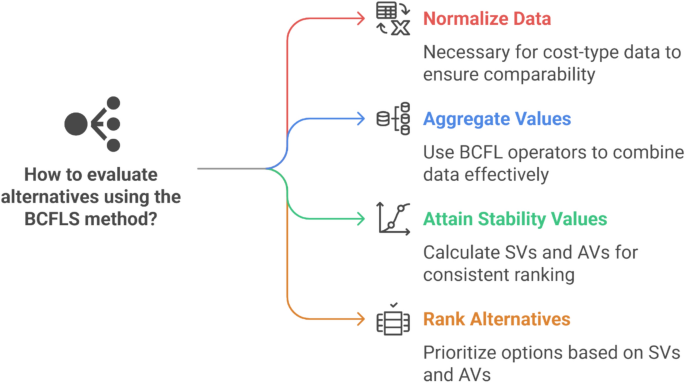
Stage 1:If the data belonging to the decision matrix is benefit sort then the normalization process is not obligatory but if the data belonging to the decision matrix is cost sort then the normalization process is obligatory and would be done by the underneath formula

在哪里，\({\left({\mu }_{P-\mathcal{Z}}\left(\mathfrak{h}\right),{\mu }_{N-\mathcal{Z}}\left(\mathfrak{h}\right)\right)}^{c}=\left(1-{\mu }_{RP-\mathcal{Z}}\left(\mathfrak{h}\right)+\iota \left(1-{\mu }_{IP-\mathcal{Z}}\left(\mathfrak{h}\right)\right), -1-{\mu }_{RN-\mathcal{Z}}\left(\mathfrak{h}\right)+\iota \left(-1-{ \mu }_{IN-\mathcal{Z}}\left(\mathfrak{h}\right)\right)\right)\)。

阶段2：This stage contains the aggregated values of the decision matrix or normalized decision matrix determined by employing one of the defined BCFLMSM, BCFLWMSM, BCFLDMSM, and BCFLWDMSM operators.

Stage 3:Attain the SV through Def (8), and in case the SVs of any two alternatives become the same, then attain accuracy value (AV) through Def (9).

Stage 4:List the ranking of alternatives relying on the attained SVs and AVs.

The flowchart of the proposed method is shown in Fig. 1。

The flowchart of the proposed bipolar complex fuzzy linguistic DM method.

Case study

Over the years, however, the healthcare industry has been experiencing a dramatic transformation, particularly in the use of artificial intelligence in diagnosis and preventive medicine.As a result of the multifactorial and multifaceted nature of disability diseases, diagnostic difficulties have long been observed in the early stages of the disease.In those chronic and complex diseases, conventional diagnostic approaches may fall short since the etiologic and pathophysiologic features are complex and not easy to detect and capture;hence, appreciated delays in their management and unfavorable patient outcomes.Disability diseases are on the increase across the world and this has called for better diagnostic techniques.As per the latest trends in epidemiological research, diseases like multiple sclerosis, Parkinson’s disease, and other neurodegenerative diseases, have been on the rise, especially among the elderly.Not only does it signal morbidity in patient populations, but also creates a significantly high cost to overall global health economies.Recent and ongoing advancements in the field of machine learning especially in artificial intelligence have created new vistas in medical science.These technologies provide capabilities that are new in the way they can identify patterns, analyze data, and make predictions.However, the healthcare sector faces a critical challenge: choosing the right AI model that can best suit disability disease prediction in this complex world.

A healthcare research institution seeks to identify the best AI model for predicting disability diseases because the selection of the model greatly influences early detection, patient care, and resource utilization.The decision expert of the healthcare research institution analyzed different AI models for disability disease prediction.After careful assessment and the first round of selection, they decided to focus on four promising approaches for medical prediction tasks, interpreted in Table1。

The evaluation of disability disease prediction models includes four AI systems which are presented in Table1。Each model offers distinct capabilities: TensorFlow Neural Network excels at handling non-linear relationships in medical data and image-based diagnosis;Random Forest Classifier demonstrates strong resistance to overfitting with excellent feature importance analysis;Support Vector Machine effectively manages high-dimensional data spaces with strong classification capabilities;and XGBoost combines multiple small prediction models to create a powerful predictive tool that performs well with unbalanced medical data.Multiple AI-based disease prediction methods exist as the leading approaches in modern medical diagnostics.

After the selection of alternatives, the decision maker very thoroughly identified the key attributes that would be used to make the evaluation.These attributes were selected following a series of consultations with medical practitioners, data scientists, and healthcare technology specialists to ensure the assessment was holistic.These attributes are devised in Table2。

describes the four essential attributes that serve as fundamental evaluation criteria for medical AI model assessment.The fundamental performance metrics that matter in medical diagnostics are measured through Prediction Accuracy by assessing sensitivity and specificity.Computational Efficiency determines the necessary resource utilization which proves essential for healthcare implementation.Medical practitioners develop trust in AI models through their ability to understand model operations.Generalizability assesses how well AI models perform when treating patients of multiple backgrounds with various healthcare backgrounds.A group of multidisciplinary experts carefully chose these evaluation attributes through consultation to establish a complete assessment framework.

As attributes contain the bipolarity and extra fuzzy information, thus, the assessment values of these AI models will be in the BCFLN that is revealed in Table3。Also, the expert interprets the weight vectors to the attributes that are\(\left(0.3, 0.1, 0.3, 0.4\right)\)。Table 3 The assessment values of AI models are interpreted by experts (hypothetical data).

presents the complete assessment values for each AI model regarding the four attributes through bipolar complex fuzzy linguistic numbers (BCFLNs).The assessment values include both positive and negative membership degrees and additional fuzzy information presented through complex numbers which provide enhanced expert evaluation capabilities.The weight vector\((0.3, 0.1, 0.3, 0.4)\)demonstrates the relative significance of each attribute where Generalizability stands as the most important followed by Prediction Accuracy and Interpretability which share equal importance, and Computational Efficiency holds the least significance.

Stage 1:As the data in Table3is beneficial sort, there is no need for stage 1.

阶段2：This stage established the aggregated values of the data portrayed in Table3by employing defined BCFLMSM, BCFLWMSM, BCFLDMSM, and BCFLWDMSM operators as described in Table4。

shows the aggregated evaluation results from applying the four proposed operators BCFLMSM, BCFLWMSM, BCFLDMSM, and BCFLWDMSM.The evaluation data from multiple dimensions gets transformed into unified comprehensive values through each aggregation approach according to the results.Each aggregation method demonstrates different priorities in evaluation criteria which produces a more well-rounded analysis than using a solitary operator evaluation approach.

Stage 3:Attained the SVs through score function and interpreted in Table5and graphically interpreted in Fig. 2。

The score values.

The score values from Table5represent the complete performance metrics of each AI model across all attributes.模型\({\mathcal{Z}}_{1}\)(TensorFlow Neural Network) produces superior performance scores of 7.776 and 1.943 when BCFLMSM and BCFLWMSM operators are utilized.The Support Vector Machine operator (Model\({\mathcal{Z}}_{1}\)) demonstrates superior performance when using BCFLDMSM and BCFLWDMSM operators but achieves this result with reduced margins.The results show that model selection choices depend heavily on aggregation methods because different operators affect which models get chosen for implementation.

The score values of each AI model appear in Fig. 1across the four aggregation operators.The performance data in Fig. 1demonstrates that Model\({\mathcal{Z}}_{1}\)stands out with BCFLMSM evaluation but displays similar results with other aggregation operators.The visual display provides action-makers with immediate recognition of performance trends as well as pairwise model ranking achievements under multiple evaluation metrics.

Stage 4:The ranking of alternatives relying on the attained SVs is shown in Table6。

The score values and ranking devised in Tables5和6provide that according to BCFLMSM and BCFLWMSM operators, the AI model\({\mathcal{Z}}_{1}\)is the most suitable one and according to BCFLDMSM and BCFLWDMSM operators,\({\mathcal{Z}}_{3}\)is the most suitable one.

The case study outcomes provide vital information about selecting AI models for disability disease prediction through detailed examination.The evaluation results show that TensorFlow Neural Network achieved top performance under BCFLMSM and BCFLWMSM operators with scores of\(7.776\)和\(1.943\)but Support Vector Machine demonstrated superior results through BCFLDMSM and BCFLWDMSM operators with scores of\(0.44\)和\(0.006\)。The selection outcomes depend heavily on the evaluation framework’s mathematical structure which demonstrates that healthcare institutions need to evaluate their specific needs when selecting evaluation methodologies.The authors stress that their approach which handles uncertainty alongside bipolarity additional fuzzy information and linguistic imprecision matches the complex medical diagnosis process where doctors manage competing priorities.The better match of decision-making methods to real-life complex situations results in more precise selection processes.Decision-makers need to implement specific multi-dimensional evaluation systems instead of standard single-factor evaluation procedures to obtain better diagnostic capacities that enhance patient results.The paragraph should appear in the “结论” section before future work discussions to establish a link between mathematical results and healthcare practicality.

灵敏度分析

Here, we analyze the sensitivity of the proposed method by changing the assessment values of the alternatives based on the criteria given in the case study.The new assessment values are devised in Table7and the new eight of each criterion are\(0.1, 0.3, 0.4,\)and 0.2 respectively.

Now to solve this data, we again use the invented method, and the result is displayed in Table8and Fig. 3

The score values of new assessment values.

The solution of new assessment values showed that by aggregating the information through BCFLMSM and BCFLWDMSM operators\({\mathcal{Z}}_{3}\)is the finest alternative and using the BCFLWMSM operator\({\mathcal{Z}}_{4}\)is the finest alternative and employing the BCFLDMSM operator\({\mathcal{Z}}_{2}\)is the finest one.We can also observe that by changing the assessment values we achieved different results.This implies that, when the data is changed the proposed approach will give different and accurate results.

This section compares the investigated theory with a few current theories depicting the defined conception of power and domination.For this purpose, we consider the approaches and AOs investigated by Wang et al.⁵², Ju et al.⁵³, Gao et al.⁵⁵, and Mahmood et al.⁴⁴and the defined approach and MSM AOs.桌子9contains the results after utilizing the considered approaches and operators, and Table10contains their ranking order.

Wang等。⁵²investigated AOs and DM approach and Ju et al.⁵⁴AOs based on MSM and DM approach in the setting of intuitionistic fuzzy LS (IFLS).The theory of IFLS can’t model the data with extra information and negative aspects.Thus, it is clear that these operators and approaches are unproductive for the data displayed in Table3。Gao等。⁵⁵investigated a DM approach in the setting of interval-valued bipolar uncertain LS (IVBULS).The theory of IVBULS can’t model the data with 2nd dimension.Thus, the interpreted approach is unproductive for the data displayed in Table3。Mahmood et al.⁴⁴investigated Hamacher AOs and DM techniques for BCFS.The theory of BCFS can model both extra information and negative aspects but in this theory, the LT is missing thus, BCFS is unproductive for data in Table3。These current approaches and operators are unproductive in the detection and diagnosis of lung cancer in a patient.The defined conception and approach are productive for the data initiated in Table1。The result is displayed in Table9along with the ranking in Table10and Fig. 4。According to BCFLMSM and BCFLWMSM operators, the patient has lung nodules and according to BCFLDMSM and BCFLWDMSM operators, the patient has small cell lung cancer.Therefore, the initiated conception is more generalized and richer.

The comparison among existing and interpreted methods.

The selection of appropriate AI models for disability disease prediction needs decision-making tools that handle various uncertainties and information types.The research addresses this essential knowledge gap through a new framework that handles various dimensions of uncertainty and complexity within DM processes.The current research delivers multiple theoretical and practical advancements to MADM research.The BCFL setting benefits from the new MSM operators which include BCFLMSM, BCFLWMSM, BCFLDMSM, and BCFLWDMSM to tackle complex DM situations.The operators demonstrate strong mathematical reliability and create an extensive structure to unite multiple information types.A comprehensive theoretical foundation exists for implementing these operators in real-world DM situations because of their characteristic analysis.The MADM technique showed better performance than traditional methods because it managed to process uncertainties alongside bipolarity and additional fuzzy information and linguistic terms simultaneously.The disability disease prediction case study demonstrated TensorFlow Neural Network as the superior choice through its score values of\(7.776\)(BCFLMSM) and\(1.943\)(BCFLWMSM) while Support Vector Machine achieved the best results under BCFLDMSM and BCFLWDMSM operators with scores of\(0.44\)和\(0.006\)分别。Our proposed method captures subtle performance differences through its\(7.776\)score difference between the TensorFlow model and SVM model operating under BCFLMSM statistically.The model ranking order under BCFLMSM and BCFLWMSM operators follows\({\mathcal{Z}}_{1}>{\mathcal{Z}}_{4}>{\mathcal{Z}}_{2}>{\mathcal{Z}}_{3}\)while BCFLDMSM and BCFLWDMSM operators produce the opposite ranking pattern of\({\mathcal{Z}}_{3}>{\mathcal{Z}}_{4}>{\mathcal{Z}}_{1}>{\mathcal{Z}}_{2}\)和\({\mathcal{Z}}_{3}>{\mathcal{Z}}_{1}>{\mathcal{Z}}_{4}>{\mathcal{Z}}_{2}\)分别。The framework shows its capability to analyze models through multiple perspectives which gives decision-makers complete insights to make technology selection decisions.This is evident from our case study on the use of AI model selection for disability disease prediction.The results indicate that our method yields more accurate and diverse evaluations than conventional methods, especially when applied to realistic medical decision-making situations.These implications are significant for theoretical research and practical use in healthcare technology management decisions.The framework we have presented gives the decision-makers a better tool to evaluate the AI models, which may result in better effectiveness in the prediction and management of disability diseases.The work presented in this paper makes a valuable research contribution both for enhancing the theoretical developments of MADM methodologies and for applying them to the selection of healthcare technology.The proposed approach can be a more suitable and accurate guide to making crucial decisions in medical technology implementation than the current methods, which may lead to enhanced patient care results due to the selection of the right AI model.

Limitation and future direction

The framework shows various limitations that reduce its effectiveness for real-time clinical implementation through its expert-driven methodology and dependent parameters.Further, the proposed work can’t handle the information of various other mathematical structures such as complex intuitionistic FS (CIFS)⁶², complex hesitant fuzzy rough set CHFRS⁶³, spherical fuzzy rough set (SFRS)⁶⁴, dual hesitant FS (DHFS)⁶⁵, etc. Thus, in the future, we aim to address these limitations and expand the proposed theories in other mathematical frameworks such as CHFRS, CIFS, SFRS, and DHFS, etc. Moreover, in the future, we would like to integrate the notion of bipolar complex fuzzy set (BCFS) and neutrosophic set to develop the notion of neutrosophic BCFS.Also, we aim to expand this work in the framework of Heptapartitioned neutrosophic soft set⁶⁶, and interval neutrosophic sets⁶⁷。

MADM:

Multi-attribute decision-making

BCFLS:

Bipolar complex fuzzy linguistic set

LTs:

Linguistic terms

MSM:

Maclaurin symmetric mean

BCFLMSM:

Bipolar complex fuzzy linguistic Maclaurin symmetric mean

BCFLWMSM:

Bipolar complex fuzzy linguistic weighted Maclaurin symmetric mean

BCFLDMSM:

Bipolar complex fuzzy linguistic dual Maclaurin symmetric mean

BCFLDWMSM:

Bipolar complex fuzzy linguistic dual weighted Maclaurin symmetric mean

DM：

决策

MD:

Membership degree

PMD:

Positive membership degree

NMD:

Negative membership degree

FS:

Fuzzy set

CF:

Complex fuzzy

BFS:

Bipolar fuzzy set

BCFS:

Bipolar complex fuzzy set

AOs:

Aggregation operators

人工智能：

人工智能

作者和隶属关系

1. Department of Mathematics, University of Management and Technology, C-II, Johar Town, Lahore, 54700, Punjab, Pakistan

   Ubaid ur Rehman

2. Department of Mathematics and Statistics, College of Science, Imam Mohammad Ibn Saud Islamic University (IMSIU), 11566, Riyadh, Saudi Arabia

   Meraj Ali Khan & Ibrahim Al-Dayel

3. King Salman Center for Disability Research, 11614, Riyadh, Saudi Arabia

   Ibrahim Al-Dayel

4. Department of Mathematics and Statistics, International Islamic University, Islamabad, Pakistan

   Tahir Mahmood

贡献

All authors contribute equal.

相应的作者

对应Ubaid ur Rehman。

Ethics declaration statement

The authors state that this is their original work, and it has not been submitted to or under consideration in any other journal simultaneously.

竞争利益

作者没有宣称没有竞争利益。

Publisher’s note

关于已发表的地图和机构隶属关系中的管辖权主张，Springer自然仍然是中立的。

开放访问This article is licensed under a Creative Commons Attribution-NonCommercial-NoDerivatives 4.0 International License, which permits any non-commercial use, sharing, distribution and reproduction in any medium or format, as long as you give appropriate credit to the original author(s) and the source, provide a link to the Creative Commons licence, and indicate if you modified the licensed material.您没有根据本许可证的许可来共享本文或部分内容的改编材料。The images or other third party material in this article are included in the article’s Creative Commons licence, unless indicated otherwise in a credit line to the material.If material is not included in the article’s Creative Commons licence and your intended use is not permitted by statutory regulation or exceeds the permitted use, you will need to obtain permission directly from the copyright holder.要查看此许可证的副本，请访问http://creativecommons.org/licenses/by-nc-nd/4.0/。重印和权限

关于这篇文章