高度适应性的深度学习平台，用于自动检测和分析囊泡胞吐作用

2025-07-12 11:59:09 英文原文

作者：Becherer, Ute

介绍

活细胞荧光显微镜在分析包括细胞器和蛋白质运动以及基于生物传感器的细胞活性的测量中起着核心作用^{1，，，，2，，，，3}。表达荧光传感器或与特定探针孵育后，通常可以将细胞活性视为记录视频中荧光强度的突然变化。尽管正在开发更灵敏，更快的系统以更快地获取大量数据，但荧光信号分析通常是一项具有挑战性的努力，需要大量的手动努力并成为瓶颈。一个明显的挑战是为细胞活动开发自动检测方法，这些方法足够通用且可靠，可以轻松实施并适用于批处理分析。

受调节的胞吐作用是细胞分泌物质必不可少的，是快速动态细胞事件的一个典型例子，该事件具有挑战性检测和测量。这个困难来自相当多的荧光信号，例如在突触传播，激素和细胞因子的释放期间，或通过免疫细胞靶向细胞毒性蛋白的靶向释放。^{4，，，，5}。一种常用的方法，是在实时成像中神经元突触传播期间发生的外生事件发生的方法，取决于用pH敏感荧光团标记的囊泡蛋白的表达，例如超级黄道素（SEP）^{6，，，，7，，，，8}或其他类型的标记物，例如亲脂FM染料^{9，，，，10，，，，11}。这些可以以不同的方式成像，包括落叶和共聚焦显微镜。要实时观察具有高时间和空间分辨率的内分泌或免疫细胞中的单个囊泡/颗粒胞吐作用，总内反射荧光（TIRF）显微镜^{12，，，，13，，，，14}与pH依赖性和独立传感器结合使用是选择的方法。TIRF显微镜使贩运和颗粒附着在质膜上的解密^{9，，，，15，，，，16}并准确地遵循它们与质膜的融合^{17，，，，18，，，，19，，，，20}。

开发在记录视频中检测外旋转事件的快速可靠系统应有助于开发精神疾病的疗法^{21，，，，22，，，，23}，糖尿病²⁴或免疫缺陷，例如淋巴淋巴结症状细胞增多症²⁵。虽然已经开发了几种自动化方法^{26，，，，27，，，，28，，，，29，，，，30，，，，31，，，，32}，他们的实际实现受到其复杂性或缺乏多种数据集的多功能性的限制。避免这些局限性的一种方法是使用机器学习，尤其是深度学习，这显然是其可靠性和有效性。深度学习应用于不同领域，例如图像分割，数据分析或3D模型预测^{33，，，，34，，，，35}。与通常只能检测特定事件的数学模型不同，可以利用适当的深度学习来区分多种类型的事件。此外，深度学习可用于开发适合各种数据的系统，从而可以最少或没有人类输入的批处理数据分析。在这里，我们介绍了一个名为IVEA的自适应自动囊泡融合检测程序（智能囊泡外胞毒性分析；发音为[ëêéªvi]），该程序使用深度学习来分析各种囊泡融合事件。IVEA是一种可训练的模块化工具，它根据计算机视觉和AI的组合使用混合方法。该程序很容易作为imagej插件访问（https://github.com/abedchouaib/ivea），并包含三个完全独立的检测/识别模块，这些模块已优化用于分析最常见的胞吐作用事件类型（补充图。 1）。

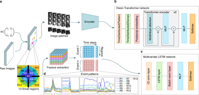
前两种技术涉及歧视神经网络，以检测荧光标记的囊泡的胞吐作用期间发生的所述爆发事件。模块ONE基于视觉变压器网络（VIT）³⁶（图 1B）在任何类型的细胞中可视化和分类单个囊泡/颗粒的胞吐作用（补充图。 1aâc）。两个模块基于一个长的短期内存（LSTM）网络³⁷由于其计算资源的需求相对较低（图 1C）。它用于检测神经元突触传播期间发生的胞吐作用（补充图。 1d，e）。第三模块旨在提取使用K-均值聚类和迭代阈值的荧光强度变化的区域（补充图。 1f，g）。

由于其模块化结构，IVEA在检测和分类的胞吐作用事件中已被证明具有特殊性和可靠性。它可以使数据以比人类专家快60倍的速度处理数据。最后，一个额外的用户友好培训平台使用户可以生成新的培训模型或完善现有的预训练模型，从而将其应用程序扩展到其他活动识别任务。

结果

用于自动分析的外生事件的分类

为了对胞吞作用进行自动分析，有必要先识别事件类别，然后创建能够识别它们的软件工具。一般而言，外囊肿事件可以分为三个主要类别（补充图。 1）。前两类与囊泡胞吐作用的测量有关（补充图。 1aâe），被视为离散点上荧光强度的短暂变化。因此，我们称这些事件，荧光爆发事件或爆发事件。当测量单个囊泡/颗粒的胞吐作用时，它们通常在胞吐作用发生前向融合部位移动（补充图。 1aâc）。该站点可以在质膜上的任何位置，在同一站点上产生多个融合。我们称这类型的事件随机爆发事件。相反，神经元的突触传播仅在突触下发生，并涵盖了短时间内多个囊泡的融合，从而导致静态位置处荧光强度的变化。这在自发性胞吐作用以及重复刺激期间都可以观察到（补充图。 1d，e）。因此，可以在不考虑移动荧光物体的情况下进行分析。第二种事件称为固定爆发事件。最后，第三类事件是由分泌发射器的测量产生的^{38，，，，39}和其他复合纳米膜^{40，，，，41}。当释放的神经递质与突触周围的纳米传感器结合时，它们会以浓度依赖性的方式发出扩散的荧光信号（补充图。 1f，g）。我们称这些事件为“热点地区”活动。检测所有这三种不同类型的事件都需要不同的分析方法（模块1 -3），涉及使用特定模型（补充表 - 1）。它们都包含在IVEA中，该IVEA在广泛使用和开源的Fiji程序中作为一个多用途插件，并在全面的GUI中使用了不同的应用程序（补充图。 2）。尽管IVEA是完全自动化的，但为用户提供了微调插件高级设置的选项（补充图。 3）或训练模型以适应特定的实验范例。事件检测和分类范例

IVEA软件分为两个阶段检测突发事件活动。

首先，它会自动识别强度波动，并在局部最大值上产生时空坐标（x，y，t）。在每个坐标周围，IVEA定义了一个感兴趣的区域（ROI），并提取一个小图像部分（例如，32â€32像素），以及在识别峰之前和之后捕获的框架（例如，每一侧10帧）（图）（图）（图） 1a）。这产生了一组集中在每个ROI上的图像贴片。在第二阶段，IVEA使用神经网络对这些图像贴片进行了分类，这些神经网络取决于爆发事件是静止的还是随机的。对于随机爆发事件（模块1），编码器视觉变压器（EVIT）处理这些图像序列以确定是否发生了胞吐作用事件（图。 1B）。由于处理大量图像贴片和扩展序列时evit的计算需求，我们实施了一个LSTM网络，用于分析固定爆发事件（模块2，图2， 1C）。在将其集成到LSTM网络中之前，图像贴片会降低维度和扁平化的过程（图。 1a，d）。此过程可以分析扩展活动序列，同时减少计算和内存开销（请参阅方法部分）。

检测和准确的预测是分析融合事件的两个关键因素。为了评估我们的软件，我们将IVEA预测与人类专家（HE）使用不同技术获得的不同视频的手动检测进行了比较。我们的结果中使用的视频没有事件在收购的最初四个帧中（请参阅方法）。

随机爆发事件的事件仿真验证（模块1）

该软件性能的初步评估是通过创建模拟视频进行的（图 2b），采用平均半径为2.7±0.36的非尺寸像素的囊泡的地面真相。通过这种方法，我们模拟了在细胞毒性T淋巴细胞（CTL）中裂解颗粒融合过程中观察到的随机爆发事件（请参阅方法）。随后，使用IVEA随机爆发事件模块分析上述视频（图 2a）使用普通计算机而不依赖GPU（请参阅方法）。除了神经网络半径外，我们采用了IVEA的默认参数，该参数设置为16个非二维像素。所有模拟的融合发生率均被成功鉴定而没有任何假阳性（FP）检测。为了确定IVEA准确性的局限性，我们在视频上引入了白噪声和泊松噪声（图 2b）使用等式。（（17）（请参阅方法部分）。

泊松噪声缩放因子α»从0.1增加到信号的10倍。我们在模拟的噪音丰富的视频上运行了ivea，并获得了99.71±0.29％的召回，精度为94.49±3.23％，F1得分为96.71±±1.91％。 2C）。当进一步增加时，由于超过信号强度的泊松噪声，IVEA开始失去一些小囊泡。对于最多1的1 =â= 10，召回率为96.86±2.55％，精度为79.22±4.68％，F1分数为86.51 – y6.51±3.27％。但是，这些是超过实验性TIRFMicroscopicy视频的噪声水平，科学家将分析。我们的结果表明，IVEA已准备好分析具有充满挑战的信噪比获得的真实数据。

随机爆发事件分析（模块1）

我们已经分析了CTL分泌裂解颗粒的几个视频（图 3a，b和补充电影 1 -4）。在CTL中，裂解颗粒是通过用荧光蛋白标记的货物蛋白颗粒剂B的表达染色的。这种荧光蛋白是pH敏感的Phuji（图 3a），弱敏感的EGFP或pH不敏感的TDTOMATO（（图 3b）产生非常不同的事件签名，如补充图中所示。 1b，c。这些视频在10分钟的持续时间内以10 hz记录，并包含1至33个CTL。在这些视频中，HE检测到的融合事件总数约为245（图 3a，b，补充电影 1 4）。用pH不敏感的荧光蛋白标记的裂解颗粒需要分析一个细胞所需的时间为10分钟，用pH敏感的荧光蛋白标记的裂解颗粒为5分钟。对于包含30个单元的视频，这相当于300分钟的分析。IVEA每个单元格需要少于一分钟的视频大小约256 -256像素和3000帧。在配备Intel Core i9 10的计算机上Th^{对于整个视频，与30个细胞无关荧光标记蛋白，这一生成总计约15分钟。}在使用不同标记蛋白的CTL数据集上进一步评估了IVEA平台的性能（图 3C）或使用小荧光标签lysotracker红色（补充图。 4）显示非常不同的融合动力学。后一个数据集是在配备不同TIRF显微镜的单独实验室中获取的。为了增加信号多样性，我们还分析了铬蛋白细胞中的随机爆发事件（图。 3D）和ins-1细胞（图 3e）分泌密集的核心颗粒。在这些细胞中，囊泡比CTL小，并且通常更包装。颗粒通过附着在荧光标记物上的NPY的过表达染色，这些标记物对MGFP或Mneongreen或Mneongreen或pH不敏感（如MCHERRY）（如MCHERRY）敏感。

为随机爆发事件的evit网络接受了10种不同类别的训练。该事件类别包括三种不同类型的胞吐作用事件：融合与散布荧光团的云，没有云的融合（突然消失）和潜在的颗粒融合（突然的融合发作）；以及其他8种类型的事件，例如快速漂移或聚焦变化，颗粒运动，随机噪声，强度波动的随机噪声，带有噪声的颗粒以及颗粒对接和撤离。通过他分析视频，在所有细胞和标签中都确定了所有视频中的770个融合事件。IVEA检测程序在156K ROI左右注册，以进行后来的分类，其中2418个由我们的EVIT网络确定为真实事件。如果随机爆发事件表现出荧光的空间扩散（补充图。 1b，c，补充电影 1 4），然后可以多次检测到一个事件（重复）。为了解决这个问题，我们设计了一种新方法，该方法随着时间的推移实现3D高斯扩展以消除冗余检测（图。 2d，等式 10）。应用我们的非最大抑制算法后 10，，，，11），选择了1025个TP事件，而1393个重复项被丢弃。因此，IVEA检测到了最初由HE确定的事件的255个事件。HE再次手动验证了所有TP事件以评估网络性能（补充表 2）。他最初因他的小事而忽略的事件很难在视觉上检测到，或者只是被忽略的事件，这可能是由于他的注意力范围有限。

我们评估了两个神经网络架构，即EVIT和LSTM，用于检测随机爆发事件分析中的胞吐作用（图。 1a，补充表 1）。HE验证了EVIT和LSTM确定的所有TP事件。分析是对所述视频进行的。根据细胞类型和颗粒标签对结果进行分配。使用的模型是Granuvision2，除了CD63-Phuji，使用了Granuvision3（图。 3）。Granuvision2模型经过训练，可以区分有和没有云的融合，而Granuvision3在两种现象上都经过训练，并结合了潜在的颗粒融合。事件周围的视觉半径是根据颗粒及其融合尺寸调节的（参见补充图。 5）。例如，使用像素大小为110 nm的视频使用14至16像素的半径（图。 3aâc），虽然半径为7至12 nm，用于像素大小为130或160 nm的视频（图 3d，e）。召回，精度，F1分数以及EVIT，LSTM和人类专家（HE）检测到的事件数量的摘要。 3（请参阅补充表 4用于统计）。

第一组代表具有pH敏感性染色的CTL（图 3a）。与HE确定的77个事件相比，结果总共产生了EVIT确定的85个TP事件，LSTM鉴定了70个事件。EVIT的最佳F1得分为97.81±0.98％（补充表 3，，，，4）。

对于代表具有pH不敏感染色的CTL的二集（图） 3b），与A HE发现的168个事件相比，EVIT检测到了219个TP事件，而LSTM确定了172个事件。EVIT的F1得分为89.31±2.12％（补充表 3，，，，4）。evit还熟练地检测到用lysotracker红色染色的裂解颗粒的胞吐作用（补充图。 4）。第三组是用于潜在颗粒融合的（图 3C

），将CTL用pH敏感的CD63-PHUJI或CD9-SEP染色。EVIT检测到96个TP事件，LSTM检测到78个，而A HE确定的86个事件。EVIT的F1得分为98.16±1.30％。

第四组包括具有挑战性胞吐作用特征的较小颗粒的铬蛋白细胞和INS-1细胞，并用pH不敏感的探针染色（图。 3D，补充图 6）。evit的表现明显优于LSTM（补充表 3，，，，4）。evit检测到的412个TP事件，LSTM检测到110，而A HE确定的292个事件。EVIT的最高F1得分为86.58±9.81％。

对于最后一组，代表使用npy-mneongreen或npy-mgfp染色的INS-1细胞（图 3e）evit确定了214个TP事件，与LSTM相比，与66相比，他检测到147个事件。EVIT的出色F1得分为93.18±2.06％，其良好是LSTM的F1分数的两倍（图。 3e，补充表 3，，，，4）。

总体而言，所有集合的平均结果表明，EVIT的表现要优于LSTM网络，因为EVIT的平均召回率为98.95±0.40％，平均精度为88.94±3.64％，平均F1得分为93.13英寸93.13英寸±±2.055％。相比之下，LSTM的平均召回率为64.87±13.18％，平均精度为86.87±3.05％，平均F1得分为68.58±10.16％。因此，我们选择选择EVIT模型作为随机爆发事件分析的IVEA软件的主要模型。

此外，我们将10届Hz视频放到1 hz中，以低图像采集频率测试IVEA性能。IVEA仍然能够在较低的频率下检测胞吐作用，但是随着采集率的降低，由于时间分辨率的减少，自然消除了快速融合事件，使它们在手动和计算上都无法检测到（补充图2） 7aâc）。

将IVEA与现有的ImageJ开源插件进行了比较⁴²。EXOJ最初是在包括CD63-Phuji和CD9-SEP标记的数据上开发和验证的，以及其他污渍，如Liu等人所发布的。⁴²。当我们在Liu等人的CD63-Phuji数据集和数据集上测试EXOJ时，EXOJ的F1得分达到88.92±7.28％，这与Granuvision3的分数相当（尽管图略低） 3C）。但是，对对pH敏感的探针进行测试时（图 3B，D和E），EXOJ没有有效检测胞吐作用事件，证明其在pH敏感的爆发事件之外的适用性有限（图。 3b，d，e）。即使对于gzmb-phuji，也对pH敏感的探针（图 3a），由于强度曲线的差异，EXOJ挣扎。我们使用默认参数对其进行了测试，然后是随后的优化过程，但是结果并没有改善（补充表） 3 5）。这表明基于规则的方法受到预定义的检测标准的约束。此外，我们测试了基于数学模型的另一个程序的Phusion⁴³。该程序没有比EXOJ产生更好的结果（请参阅补充表 6）。

EXOJ在特定类型的胞吐作用（潜在颗粒融合）上表现出与IVEA相当的出色性能，同时未能检测到其他类型。相反，由EVIT提供支持的IVEA的基于深度学习的方法成功地证明了在pH敏感和pH不敏感数据集中检测胞吐事件的能力。通过通过新训练学习复杂的时空模式，或通过改进过程来调整预训练的模型，示例适应了各种荧光信号（补充图。 8）。通过在心肌细胞中用氟4测量的30个钙火花事件上的30个钙火花事件上的颗粒颗粒3⁴⁴，与改进之前的200相比，我们能够检测到298 TP和2个FP事件。这使IVEA成为一种非常多功能且可靠的检测框架，适合于更广泛的实验条件。

IVEA的输出由两个文件集组成：一个ImageJ ROI ZIP文件和两个分析CSV文件。每个ROI在其对应的事件的荧光强度的峰值处标记并位于质量中心。CSV文件包含在固定时间间隔内的每个事件的荧光强度的测量\（x \）和\（y \）center of mass coordinates, their full width at half maximum (FWHM), and the fluorescence intensity kinetics (rise time, decay and temporal FWHM).

Stationary burst events analysis (module 2)

Stationary burst events were analyzed using the second branch of our platform (Fig.Â 4a), which employs the LSTM neural network for classification (Fig.Â 1a, c, Supplementary TableÂ 1）。The rationale behind this choice was conservation of memory and computational power.Our eViT for random burst events requires an input sequence of 26 image patches with a size of 32â€‰Ã—â€‰32 pixels.This necessitates high memory and computational power both during the training phase and classification task.In the case of stationary burst events, the number of frames per sequence required to analyze an exocytosis event would need to be significantly higher than for random burst events due to different signal kinetics.A reasonable number of frames to study them would be between 41âˆ’100 frames.Furthermore, the number of selected regions to extract the image patches is high, with up to 14,000 ROIs in a single video.This would result in huge memory demands, necessitating the use of high-end computational resources to analyze stationary burst events with our current eViT.

**Fig. 4: Detection and analysis of exocytosis in neurons with stationary burst event algorithm.一个**

We analyzed DRG neurons videos expressing SypHy that were derived from Shaib et al.⁴⁵and Staudt et al.⁴⁶。These videos display a variety of synapse count, intensity, vesicle movement, and background activity.In our data set, stationary burst events were characterized by fast rise (within 4.1 s, i.e. 41 frames acquired at 10â€‰Hz, Supplementary Fig.Â 9d) of the fluorescence intensity in a spot like area (Supplementary Fig.Â 10a）。Our neural network input layer for the stationary burst events was adapted for the input vector${{{\bf{P}}}}\left({{{\bf{x}}}}\left(t\right){{,}}{\mathfrak{f}}\right)\in {{\mathbb{R}}}^{T\times {\mathfrak{f}}}$，在哪里${{{\bf{x}}}}\left(t\right)\in {{\mathbb{R}}}^{T}$作为${\mathfrak{f}}$is the number of regions and$t$is the time series for$0 < t\le T=41$和$t\,{\mathbb{\in}}\,{\mathbb{N}}$。Thus, the LSTM network discards the majority of the selected eventsÂ stored whithin matrix${{{\boldsymbol{{{\mathscr{W}}}}}}}^{{\prime} }$(i.e. the selected regions, Fig.Â 1a) resulting in the classification of highly probable true events.For events in which the rise time was longer than 41 frames, the LSTM network sorted the events into the â€œintensity riseâ€ category (Supplementary Fig.Â 9C) thereby discarding them from the collection of true events.For experimental conditions in which long lasting events with slow kinetics are the result of long stimulation paradigms or very high acquisition frequency (Supplementary Fig.Â 10), we adapted an â€œadd frameâ€ option that allows the user to adjust the eventâ€™s time window by increasing the number of frames by${t}_{n}$(see method section).The videos that were analyzed, were acquired at 10â€‰Hz and comprised 3000 frames, each measuring either 512 by 512 pixels⁴⁵or 512 by 256 pixel⁴⁶。The DRG neurons were stimulated electrically for 1 min⁴⁵or they were stimulated twice for 30â€‰s and 1â€‰min with 10â€‰s recovery phase in between⁴⁶。The human analysis of these videos was a challenging task that required an average of 60â€‰min per video.Detected events had predominantly a high fluorescence intensity variation or lasted for relatively long periods of time.IVEA reduces the time of analysis of the same videos to under 1â€‰min per video.Furthermore, batch analysis capabilities exclude the need for manual parameter adjustment, as the tool automatically adapt to the input videoâ€™s characteristics.

The results of the analyzed videos show that the neural network was able to classify virtually all the human labeled regions (Fig.Â 4b, c）。Additionally, the neural network was able to detect more true fusion events than HE had originally detected by double checking and validating them as real events.The HE was able to detect overall 356 fusion events, while IVEA detection routine registered 84k ROIs for later classification.Most of these events were identified by the neural network as false events.A total of 2049 events were classified as true events, while only 70 events were identified as FP (Fig.Â 4C）。The average recall, precision and F1 score were 88.12â€‰Â±â€‰2.70%, 96.37â€‰Â±â€‰0.45%, and 91.83â€‰Â±â€‰1.61% respectively.Importantly, in comparison to the HE approaches, the LSTM network for stationary burst events could detect weak events or events with fast kinetics (Supplementary Fig.Â 9e, f;Supplementary MovieÂ 5）。Conversely, the HE was able to detect events with very slow kinetics (Fig.Â 4b) (Supplementary Fig.Â 10b）。Due to the â€œintensity riseâ€ category (Supplementary Fig.Â 9C) these slow events (i.e. longer than 41 frames) were missed by IVEA in the videos from Staudt et al.⁴⁶, in which long stimulation paradigms were applied to the cells, yielding more long-lasting events.However, they were detected when applying the â€œadd frameâ€ option that extends the time interval by adding 60 frames for correct classification (Supplementary Fig.Â 10, Supplementary MovieÂ 5）。Overall, IVEA identified about 5.4â€‰times as many true events as HE.We compared IVEA to the existing open source software SynActJ³²that was devised to analyze synaptic activity in neurons stained with the overexpression of synaptobrevin-SEP or alike proteins.First, we compared the result of IVEA and SynActJ on the provided test movie.SynActJ and IVEA were able to identify most of the active synapses but missed one and yielded one FP event (Supplementary Fig.Â 11a）。Then, we compared both programs on one of our movies in which synaptic activity was clearly detectable by HE.While IVEA detected all events without any FP events, SynActJ was able to detect only a very limited number of active synapses and showed a significant number of FP events (Supplementary Fig.Â 11b）。Thus, IVEA is by far superior to SynActJ.

For advanced analysis, IVEA distinguishes between various event types and categorize them based on their timing in respect of the experimental stimulation paradigms.The events can be classified as synchronized to the stimulus or unsynchronized (Fig.Â 4C）。This feature was implemented as both types of events might show differences in kinetics.Stimulation time can be set manually, but to ease usability we also implemented an automatic stimulation detection.Our neural network was trained on${n}_{c}=9$distinct events categories.These categories include: four types of events (fusion, short time fusion$\sim 4$frames (0.4â€‰sec at 10â€‰Hz), electrical or agonist stimulation, and NH4₊^{treatment) and five types of artifacts (fluorescence intensity rising, out-of-focus artifacts, vesicle motion, white noise, and fluorescence intensity fluctuations).}While events are sorted and labeled, spatial recognition task is performed to locate and unify the eventâ€™s spatial identity while counting how many times the same synapse was active.

Finally, the output for the stationary burst events are ROIs files whereby each ROIs is positioned at the eventâ€™s maximum intensity temporal occurrence.The ROIs are labeled with an ID, frame number and event status.Additional outputs are the summary for each event and the measurements, such as intensity over a specified time interval and over the full video length.

Hotspot area extraction (module 3)

For the third analysis conducted using IVEA, we employed distinct techniques from those mentioned earlier.In this analysis, we assumed that the sensor array was in a fixed position, awaiting the occurrence of hotspots.Due to the limited availability of training data and the simpler features compared to the stationary and random burst events, we opted not to implement a neural network.Instead, we utilized k-means clustering and iterative thresholding for detection, and employed spatial search with mean intensity tracking over time for event recognition (Fig.Â 5a）。Before applying the foreground detection method, we perform intensity fluctuation correction.The challenge while correcting the intensity fluctuation is to avoid altering and distorting the event as much as possible.To address this, we have developed a new method utilizing k-means combined with simple ratio for pixels value grouping and adjustment (see Methods).We call it â€œMultilayer Intensity Correctionâ€ (MIC) (Supplementary Fig.Â 12）。The main idea of our method is to perform pixel value correction based on the variation of the average value of each cluster of pixels.To preserve the signal intensity, the signal should be a small range of pixels registered in a cluster, otherwise the signal is affected by the average value adjustment.MIC algorithm is performed through segmenting a given image into$k$layers using the k-mean clustering algorithm⁴⁷after performing Gaussian filter of sigma equal to 1. After performing foreground detection, we extracted the hotspots from the processed image$\Delta I$by converting it to a binary image using a global threshold (Fig.Â 5b）。自从$\Delta I$is the resulting matrix of intensity variation between two images, applying different types of threshold algorithms specially those found in Fiji, lead to unpredictable results.Therefore, we implemented our own iterative global threshold (Fig.Â 5c）。The iterative threshold is not dependent on the statistical information calculated from the image.Instead, it is iterated over the noise level$\Delta I$, with the objective of eliminating it (Fig.Â 5b）。This allows us to determine the global threshold for the fluorescence intensity value (see Methods).After detection of the possible hotspot, the fluorescence intensity of each event is temporally tracked (Fig.Â 5d）。When the fluorescence intensity of the event falls below the mid intensity, the event signal is considered to have disappeared and the tracking stops (Fig.Â 5e）。The IVEA software, which uses advanced algorithms and automated parameters, reduced the need for users to iteratively adjust the parameters for analysis.Furthermore, it enhances precision compared to the previously used DART software with default parameters (Fig.Â 5f）。

**Fig. 5: Overview of the sensor-based exocytosis detection algorithm.一个**

讨论

IVEA is a robust, pre-trained plugin for activity recognition, dedicated to the detection and analysis of vesicle exocytosis.It seamlessly integrates into the Fiji platform for open-source accessibility.IVEA achieves an impressive performance with F1 scores as high as 98â€‰Â±â€‰1% for the eViT (random burst events, Fig.Â 4) and 94â€‰Â±â€‰1% for the LSTM neural network (stationary burst events, Fig.Â 5）。Furthermore, IVEA is proficient in distinguishing real events from artifacts such as photon shot noise or fast transient focus change (Supplementary Fig.Â 9a）。Three different algorithms can be selected by the user, making IVEA highly compatible with a range of exocytotic events displaying varying fluorescence intensity profiles (Supplementary TableÂ 1）。Additionally, IVEAâ€™s high adaptability results from its machine learning foundation, particularly, leveraging deep learning ViT³⁶, CNN and sequential models⁴⁸。This enables IVEA to not only identify a wide range of exocytosis events, but also to learn and recognize new patterns, thereby expanding the scope of its capabilities.

Other Fiji-based exocytosis analysis plugins such as PTrackII³¹SynAct³²or ExoJ³⁰已经开发了。Their algorithms rely on fixed mathematical and/or morphological models that are proficient at detecting a limited range of events as these algorithms cannot adapt and learn by themselves.The detection parameters can be adapted to a certain degree by adjusting complex input parameters that can be overwhelming for users with limited programming skills.This also precludes easy implementation of batch analysis when the analyzed videos have different characteristics, such as varying noise levels or fusion kinetics.Other programs like pHusion, have been developed but are only available in MATLAB, Python, or other proprietary platforms, making them less accessible^{27，，，，28，，，，29，，，，43}。Finally, an algorithm has been developed with the variability of the signal in mind, using convolutional neural network (CNN)²⁶, which is not made available as a software.In contrast, IVEA â€“ a â€œplug and playâ€ plugin, distinguishes itself by the adaptability of the detection and classification capabilities that is based on multivariate LSTM⁴⁹and ViT³⁶型号。For stationary burst events, we chose LSTM network for the analysis, as it requires less memory usage when compared to eViT.This is particularly important as the number of extracted sequence patches and the number of frames analyzed per sequence is high.An analysis of all these sequences by eViT would require huge computational resources that cannot be provided by CPU computation and a reasonable RAM size (about 64 GB).In contrast, for random burst events, the presence of motion and other variables makes the classification of the events complex.This necessitates the use of more sophisticated models, such as the ViT network.To support this model, an encoder network was adapted and implemented to extract features prior to the ViT network.The added layers to the ViT model³⁶was demonstrated using an ablation study (Supplementary Fig.Â 15) (see Method).

To assess IVEAâ€™s versatility, we extensively trained and evaluated it on exocytotic events in CTL, chromaffin cells, INS-1 cell and DRG neurons.Consequently, we were able to detect exocytotic events with high effectiveness, achieving a recall of 98â€‰Â±â€‰4% and F1 score of 90â€‰Â±â€‰6%, even in videos with low SNR and events presenting minimal features (dense core granules in INS-1 cells labeled with the pH-insensitive NPY-mCherry).Additional challenges such as granule clustering do not impair IVEAâ€™s capability to identify weak exocytotic events (Supplementary Fig.Â 6）。Finally, IVEA successfully detected exocytotic events with different signatures than those used for training, albeit with some additional FP (Supplementary Fig.Â 4）。However, IVEA is not designed to detect non-burst events such as those recorded in hippocampal neurons labeled with Synaptobrevin-SEP, FM1-43 or CypHer5E.In the case of Synaptobrevin-SEP stimulated exocytosis at synapses results in long-lasting increased fluorescence spreading out of the synapse^{50，，，，51}, while with FM1-43⁵²and CypHer5E⁹, it produces only a very slow decay of fluorescence.In the future, adapting the eViT capability and retraining the new neural network may enable this type of analysis.However, this will require advanced computational capabilities and different dataset labeling.In contrast, we foresee that IVEA would have minimal difficulty of detecting synaptic transmission measured via iGluSnFR3⁵³。While IVEA is virtually universal for detecting burst exocytosis in a wide array of experimental paradigms with the current trained models, users might still encounter specific needs.Therefore, we provide Python scripts with a simple GUI for training purposes, along with a configuration JSON file for parameter adjustments.The choice to use Python was motivated by challenges related to vectorized computations, alongside variations in the versions of C++ jar files across Fiji, Google TensorFlow, and the deeplearning4J library.These scripts facilitate the training of a new model and the implementation of transfer learning by freezing the majority of neural network layers and retaining the last two Dense layers of the eViT⁵⁴。This refinement of an existing eViT model reduces the time required for training and the labeling of data³⁴。Additionally, it can be trained on a central processing unit (CPU) rather than a graphics processing units (GPU).

IVEA shows robust analysis capability even when the noise power is equal to that of true events by extracting spatiotemporal features of the signal (Fig.Â 2C）。Additionally, IVEA is capable of discarding artifacts such as short focus changes resulting in transient signal variation.However, slow focus drift cannot be compensated as well as lateral drift in the case of stationary burst events.Upon drift an active synapse is detected at different locations and is assigned to several coordinates.Therefore, drift should be corrected using free plugins such as but not limited to NanoJ core⁵⁵prior to IVEA analysis.Random burst event does not require drift correction as the algorithm does not require fixed spatial coordinates.Finally, to detect exocytosis events, the IVEA algorithm requires analyzing the first four frames from each video.This step is important for the automation process, so that IVEA can learn from the images that are devoid of events (see method section â€œstationary and random burst events algorithmâ€).In rare cases in which videos contain events within these frames, IVEA can generate learning parameters that enable the detection of high SNR events while events with low SNR may be overlooked.However, manually reducing the detection threshold to 1 or less can enhance the sensitivity of event selection.The neural network can classify these increased detections correctly, while eliminating most of the FP events.As a result, a heightened computational time requirement may arise.This can be mitigated by extracting more than four frames that are devoid of events and adding them to the beginning of the movie.

In conclusion, IVEA reduces analysis time by >90%, requiring minimal to no human input, and significantly decreases analysis bias.Furthermore, the number of fusion events detected by IVEA is higher than those detected by the human expert, especially when it comes to visualizing rare, i.e. low brightness, events in low-SNR conditions.This allows us to generate large datasets with meaningful statistical power.In addition, IVEA unlike the human expert readily detects short events, which not only increases the number of detected events but also promotes the understanding of biological processes.The earlier application of hotspot area extraction module for AndromeDA revealed not only discrete dopamine (DA) release and extracellular DA diffusion, but it also enabled the discovery of heterogeneous release hotspots - albeit using a less-advanced algorithm at the time.The trove of information collected from individual events allowed to elucidate the role of key proteins in the molecular machinery of exocytosis in dopaminergic neurons³⁹。

We foresee that our program will be adaptable to analyze exocytosis in many other systems and to extend its use to other burst-like events.For instance, the eViT method with additional training was proficient at analyzing transient localized calcium signals with low SNR, such as calcium sparks.The â€œhotspot area extractionâ€ should be capable of analyzing calcium waves in cell clusters, brain slices or in vivo measurements.Using IVEA for detecting exocytosis events has the potential to rapidly advance research in the neuroscience, immunology, and endocrinology.

方法

Stationary and random burst events algorithm

Our approach to detecting burst events involves two main parts: automatic region selection and neural network classification.The first part is detecting the potential ROIs.The event detection algorithm used by IVEA employs the grayscale image foreground detection method, which leverages a bidirectional image subtraction technique.This involves subtracting the intensity values in a 16-bit image stack of a reference frame${I}_{i}$from an offset frame${I}_{i+n}$in both directionsâ€”forward$(\Delta {I}_{F}={I}_{i+n}-{I}_{i})$and backward$(\Delta {I}_{B}={I}_{i}-{I}_{i+n})$。This approach simplifies the handling of 32-bit matrices, reducing potential complexities with straightforward data processing.Backward subtraction is employed only with random burst events to detect fusion events visualized with a pH-insensitive stain.In the absence of fluctuations or foreground variations, the subtraction results in an image with pixel values of zero.However, the presence of noise and/or artifactual fluctuations during image acquisition makes it difficult to differentiate real events from artifacts.To distinguish real events from noise, we detect local maxima (LM) in the subtracted images, representing potential exocytic hotspots.Subsequently, an ROI is generated around each identified LM.These ROIs are then employed to generate image patches, which correspond to cropped sections of video frames.This approach captures localized activities over time, thereby enabling the isolation of specific events for classification rather than analyzing the entire video frame-by-frame with the neural network.The LM detection and ROI extraction process is fully automated, incorporating a global thresholding step that learns from the first four frames of the processed video.This ensures that noise and spurious maxima are filtered out, leaving only meaningful events for classification.The local minima prominence${{{\mathcal{p}}}}$approximation algorithm iterates over the noisy images;each iteration increments the value${{{{\mathcal{p}}}}}_{n}$until the number of LM coordinates (${l}_{n}$) equals 0. If, instead, four successive iterations yield the same number of maxima (e.g.,${l}_{n}=\,{l}_{n-4}$), the program sets${{{\mathcal{p}}}}={{{{\mathcal{p}}}}}_{n}$where â€œ$n$â€ is the iteration number.These four images are also utilized to estimate the full width at half maximum (FWHM)$\sigma$of the noise LMs, and to measure$\Delta \mu$, which is the average of the mean intensities$\Delta {\mu }_{j}$at LM${C}_{j}$with radius$r$expressed as:

$$\Delta {\mu }_{j}=\frac{1}{4{r}^{2}+1\,}{\sum }_{{C}_{j}^{(x)}-r}^{{C}_{j}^{(x)}+r}{\sum }_{{C}_{j}^{(y)}-r}^{{C}_{j}^{(y)}+r}\Delta {I}_{i}({x}_{j},{y}_{j})\,{with}\,{r}\,{\mathbb{\in}}\,{\mathbb{N}}$$

（1）

The region selection procedure is similar to parameter automation.We determine$\Delta {\mu }_{j}$和${\sigma }_{j}$for each event${E}_{j}$在${C}_{j}$。To designate${E}_{j}$as a selected region we employ the following condition:

$${E}_{j}\left|\left(\Delta {\mu }_{j} > \Delta \mu \cdot \theta \right)\wedge \left({\sigma }_{j} > \sigma \right)\,{with}\,\sigma,\theta \,{\mathbb{\in }}\,{\mathbb{R}}\right.$$

（2）

Here, Î¸ denotes the sensitivity parameter, which can be adjusted by the user.

After detection, IVEA performs spatiotemporal tracking for ROI recognition and labeling.This is applied for each detected ROI coordinate over a certain radius and period.For burst events exhibiting temporal dynamics (e.g., lytic granule fusion), a sequence of image patches is extracted, encompassing frames both preceding and following the time point of the event.Each sequence is fed to a shared encoder layer attached to the ViT architecture for image recognition as described in Dosovitskiy et al.³⁶。We designated the modified architecture as eViT.The image patchesâ€™ spatial dimensions are variable, but they are scaled to fit the encoder input layer of 32â€‰Ã—â€‰32 dimensions.Each patch represents the extracted area centered at the LM, while the sequence is centered on the fluorescence intensity peak time (Fig.Â 1a）。The encoder network automatically extracts features from each sequence and forwards the encoded data to a multi-layered perceptron (MLP), which in turn forwards the data to the ViT network.The ViT network then performs positional encoding on the extracted features and classifies each sequence as a true event or not (Fig.Â 1B）。

For stationary burst events, we employed a straightforward model architecture comprising an LSTM network³⁷for exocytosis classification.Our LSTM architecture is designed for multivariate time series classification⁴⁹(Fig.Â 1C）。In this case, the image patches undergo feature extraction preprocessing to convert them into one-dimensional time-series vectors (Fig.Â 1a）。These feature vectors are subsequently fed into the LSTM network for classification (Fig.Â 1d）。An additional optional method is implemented in the stationary burst events for detecting and tracking agonist/electric and NH₄⁺stimulations.This algorithm is utilized to recognize and sort events based on their occurrence period.Stimulus detection is expressed as:

$${{{{\mathcal{R}}}}}_{i}=\frac{\Delta {\mu }_{i+1}}{\Delta {\mu }_{i}}\, > {\theta }_{s}$$

（3）

在哪里${{{{\mathcal{R}}}}}_{i}$is the mean ratio;${\theta }_{s}$is the default threshold, is 1.1;$\,\Delta {\mu }_{i}$和$\Delta {\mu }_{i+1}$are the mean gray value of image$\Delta {I}_{i}$和$\Delta {I}_{i+1}$分别。

To avoid an increase in the number of detected events due to high fluorescence intensity during the stimulus period, we adjust the detection sensitivity by increasing the detection sensitivity${\theta }_{i}$，例如${\theta }_{i}=\theta \cdot {{{{\mathcal{R}}}}}_{i}$。

Feature extraction

Feature extraction is performed by extracting a sequence of image patches around${C}_{j}$over a time interval.This patch is subdivided into smaller regions.Subsequently, we determine the mean intensity of each region (Fig.Â 1a）。For each selected region denoted as${E}_{j}$, we extract the spatial neighboring pixels around${C}_{j}$as a 2D matrix${{{{\bf{M}}}}}\,^{j}\in \,{{\mathbb{R}}}^{k\times k}$，在哪里$k$is the kernel defined by the user.The spatiotemporal data${{{{\bf{V}}}}}_{j}\in \,{{\mathbb{R}}}^{k\times k\times T}$, which represents event${E}_{j}$that occurred at time${t}_{j}$, is extracted over several frames T expressed as (3).

$${{{{\bf{V}}}}}_{j}\left(x,y,t\right):\!\!=\left\{{{{{\bf{M}}}}}_{t}^{j}\left(x,y\right)\, \left|\,t\in \left[{t}_{j}-{n}_{b},{t}_{j}+{n}_{a}\right]\right.\right\}$$

（4）

然而${n}_{b}$is the number of frames before${t}_{j}$和${n}_{a}$is the number of frames after${t}_{j}$。The spatial coordinates of each matrix${{{{\bf{M}}}}}\,^{j}$are split into 13 small regions${\mathfrak{f}}\,\epsilon \,{\mathbb{N}}$(see Supplementary Fig.Â 13a), which yield the feature matrix${{{{\bf{P}}}}}_{j}\,\epsilon \,{{\mathbb{R}}}^{T\times {\mathfrak{f}}}$事件${E}_{j}$such as (4):

$${{{{\bf{P}}}}}_{j}\left({{{\bf{x}}}}\left(t\right){{,}}{\mathfrak{f}}\right):\!\!=\left\{\frac{1}{{n}_{f}}{\sum }_{f=1}^{{n}_{f}}{{{{\bf{V}}}}}_{j}\left({x}_{f},{y}_{f},t\right) |\,f\in \,\left[1,{\mathfrak{f}}\right]\right\}$$

（5）

然而${n}_{f}$is the number of pixels in each region$f$。

This approach forms time series data${{{\bf{P}}}}$, represented as${{{\bf{P}}}}\in {{\mathbb{R}}}^{{n}_{s}\times T\times {\mathfrak{f}}}$，在哪里${n}_{s}$is the total number of nominated events.Each element${{{{\bf{P}}}}}_{j}$在${{{\bf{P}}}}$represents 13 distinct signals that capture the fluorescence intensity profile of different regions plotted on a single graph (Fig.Â 1d, Supplementary Fig.Â 9）。The choice of small, symmetrical regions over circular masks enhances feature preservation of the spatiotemporal signal (Supplementary Fig.Â 13a, c）。Additionally, we opted for 13 regions over 9 regions due to their higher sensitivity in capturing slow granule movements (Supplementary Fig.Â 13a, b）。

If the number of frames increases by${t}_{n}$，例如${{{{\bf{x}}}}}^{{\prime} }\left(t\right)\in {{\mathbb{R}}}^{{{{\mathcal{t}}}}}$和${{{\mathcal{t}}}}=T+{t}_{n}$。${{{\bf{P}}}}\left({{{\bf{x}}}}\left(t\right){{,}}{\mathfrak{f}}\right)\in {{\mathbb{R}}}^{T\times {\mathfrak{f}}}$is then determined by using windowing mean-sampling expressed as:

$${{{\bf{x}}}}{\left(t\right)}_{i}=\left\{\frac{1}{{{{\mathcal{w}}}}}{\sum }_{k=1}^{{{{\mathcal{w}}}}}{{{{\bf{x}}}}}^{{\prime} }{\left(t\right)}_{{{{\mathcal{w}}}}\left(i-1\right)+k}\, \right|{{{\mathcal{w}}}}=\frac{{{{\mathcal{t}}}}}{T}\,{with}\,{{{\mathcal{w}}}}\,{\mathbb{\in}}\,{\mathbb{N}}$$

（6）

在哪里，${{{\bf{x}}}}{\left(t\right)}_{i}$是$i-{\mbox{th}}$element of the sampled vector${{{\bf{x}}}}\left(t\right)$，和${{{{\bf{x}}}}}^{{\prime} }{\left(t\right)}_{j}$作为$j=\,{{{\mathcal{w}}}}\left(i-1\right)+k$是$j-{\mbox{th}}$element of vector${{{{\bf{x}}}}}^{{\prime} }(t)$。

For stationary burst events, we used${n}_{b}=10$和${n}_{a}=30$time samples, resulting in a total of$T=41$time samples.For random burst events, the implemented LSTM model used a total number of time samples$T=21$（（${n}_{b}=10$和${n}_{a}=10$）。The time series data${{{\bf{P}}}}$is first normalized within the range of 0 to 1 before being converted to tensors.For stationary burst events analysis,${{{\bf{P}}}}$is converted into 3D tensors${{{\boldsymbol{{{\mathcal{T}}}}}}}\in {{\mathbb{R}}}^{{n}_{s} \times {\mathfrak{f}} \times {T}}$as follows:

$${{{\bf{P}}}}\left(j,{{{\bf{x}}}}\left(t\right){{,}}{\mathfrak{f}}\right)\to \,{{{\boldsymbol{{{\mathscr{T}}}}}}}\left(j{{,}}{\mathfrak{f}}{{,}}{{{\bf{x}}}}\left(t\right)\right)\,|\,j\in \left[1,{n}_{s}\right]{with}\,{n}_{s} \,,j\,{\mathbb{\in }}\,{\mathbb{N}}$$

（7）

Multivariate LSTM neural network architecture

Our LSTM network comprises four different layers.It serves as a robust framework for multivariate temporal data analysis.The first input layer, defined by the input-shape specification, establishes the dimensions of the incoming multivariate time series data.This initial stage isnâ€™t a distinct processing layer but rather a configuration step to align the network with the input dataâ€™s structure.The subsequent architecture unfolds with a 1D convolution layer employing Rectified Linear Unit (ReLU) activation function.The subsequent layer incorporates a LSTM, designed to recognize sequential patterns.To promote stable training dynamics, a batch-normalization layer is added.The last layer is the fully-connected Dense layer that employs the softmax activation function, rendering the architecture adept for multiclass classification.

$${\hat{{{{\mathcal{y}}}}}}_{i}=h\left({{{\mathcal{z}}}}\right)=\frac{{e}^{{{{{\mathcal{z}}}}}_{i}}}{{\sum }_{j=1}^{{n}_{c}}{e}^{{{{{\mathcal{z}}}}}_{j}}}$$

（8）

这里，${h}\left({{{\mathcal{z}}}}\right)$is the softmax function,${{{{\mathcal{z}}}}}_{i}$represents the raw score (logit) for a specific class\（我\）和${n}_{c}$is the number of classes.This arrangement encapsulates both localized and temporal patterns inherent to multivariate sequential data, combining convolution, recurrent, and normalization mechanisms.The network is structured to accommodate categorical cross-entropy as the loss function${{{\mathcal{L}}}}$(Eq.Â 9), tailored for multiclass categorization, while optimization leverages the Adam optimizer with a learning rate of$3\times {10}^{-4}$。

$${{{\mathcal{L}}}}=\frac{1}{{n}_{s}\,}{\sum }_{j=1}^{{n}_{s}\,}L\left({\hat{{{{\mathcal{y}}}}}}^{(j)}\right),{{\mbox{with}}}\,L\left({\hat{{{{\mathcal{y}}}}}}^{(j)}\right)=-{\sum }_{i=1}^{{n}_{c}}{{{{\mathcal{y}}}}}_{i}^{\left(j\right)}\cdot \log \left({\hat{{{{\mathcal{y}}}}}}_{i}^{\left(j\right)}\right)$$

（9）

在哪里$L\left({\hat{{{{\mathcal{y}}}}}}^{(j)}\right)$is the loss for a single data point (sample),${n}_{s}$is the number of data points,${{{{\mathcal{y}}}}}_{i}$ $\in \left\{0,\,1\right\}$is the true label for class\（{我}\）和${\hat{{{{\mathcal{y}}}}}}_{i}$is the predicted probability.

Encoder-ViT network architecture

Our eViT network consists of two components: a CNN as the encoder for feature extraction from image patches and a ViT for classification.The encoder is shared CNN.It comprises seven layers, including a 2D spatial convolution layer that is followed by a sequence of 3D convolution layers and 3D max pooling operations (Supplementary Fig.Â 14a, b）。

We have two pre-trained models available with IVEA, namely GranuVision2 and GranuVision3.The modelâ€™s encoder input layer accepts time series image patches of length 26 for GranuVision2 and 28 for GranuVision3.The width, height and channel of each patch is 32â€‰Ã—â€‰32â€‰Ã—â€‰1, denoted as${{{\bf{X}}}}\in {{\mathbb{R}}}^{t\times w\times h\times c}$。If the dimensions of the image patches change, we use bilinear interpolation to resize the images to 32â€‰Ã—â€‰32.The initial stage of the shared CNN involves the application of a 3D convolution layer with 16 filters and ReLU activation, which is followed by a 3D max pooling layer.Subsequently, another 3D convolution layer with 32 filters and ReLU activation is applied, followed by a 3D max pooling layer.Finally, a 3D convolution layer with 64 filters and ReLU activation is applied, followed by a 3D max pooling layer.The output of the encoder is passed through a Flatten layer and a 64-unit Dense layer.Positional embeddings are added before the sequence enters the transformer block, which includes an MLP.The transformer block consists of multi-head self-attention and an MLP, each with a residual connection (Fig.Â 1B）。The transformer block operates on an input sequence of length equal to the time series dimension, with a key dimension representing the output size of the previous Dense layer.The MLP inside the transformer block consists of two Dense layers, where the first layer has a dimension twice the key dimension, and the second layer projects it back to the key dimension.The final MLP comprises two Dense layers: the first layer with GELU non-linearity, and the second with SoftMax activation, classifying 10 (2 fusion + 8 artifacts) or 11 (3 fusion + 8 artifacts) classes for GranuVision2 or GranuVision3, respectively.The eViT architecture underwent ablation to study the impact of layers on model performance.This study involved probing the model on an evaluation dataset by eliminating layers and retraining.The evaluation dataset was divided into two categories: exocytosis (positive labels) or non-exocytosis (negative labels).We performed the ablation study on the shared CNN layers and the penultimate Dense layer.The results show that progressively removing these layers leads to a noticeable decline in performance.The final configuration, with only one convolution layer, exhibited the strongest performance drop.This study underscores the additive role of each layer in our current eViT architecture (see Supplementary Fig.Â 15）。

Gaussian non-max suppression

Various non-maximum suppression techniques are typically used to address the multiple overlapping-detections problem, including the classical intersection over union (IoU) method, weighted boxes fusion (WBF), and others⁵⁶。However, these methods cannot be implemented with our data because exocytotic events cannot be limited to objects with boundaries or boxes.Thus, we have developed a new method that implements 3D Gaussian spread over time

$$g\left(x,y,t\right)=\Delta {{{\rm{\mu }}}}\cdot \exp \left(-\frac{\left(\Delta {x}^{2}+\Delta {y}^{2}\right)}{2{\left(\sigma+{SR}\right)}^{2}}\right)\cdot \exp \left(-\frac{\Delta {t}^{2}}{2{\tau }^{2}}\right)\,{with}\,\tau={{{\mathcal{v}}}}{\mathscr\,{\cdot }}\,\sigma$$

（10）

在哪里$\Delta {{{\rm{\mu }}}}$is the fluorescence intensity of the event area in the subtracted image;$\sigma$is the eventâ€™s cloud spread;${\mbox{SR}}\,=1$is a user-controlled spread radius;$\tau$is the temporal cloud spread;和${{{\mathcal{v}}}}$is the image acquisition frequency set to 10â€‰Hz.

To isolate prime events from redundant ones, we apply$g\left(x,y,t\right)$to each pair of events as follows:

$$\left\{\begin{array}{cc}{E}_{i}={E}_{j}&{{{\rm{if}}}}\,\Delta {\mu }_{i} < {g}_{j}\left({x}_{j},{y}_{j},{t}_{j}\right)\,\hfill \\ {E}_{i}\,\ne {E}_{j}&{\mbox{otherwise}}\,\end{array}\right.$$

（11）

在哪里${E}_{i}$和${E}_{j}$are two different true positive (TP) events.

Neural network training and evaluation

Python was utilized for developing and training the LSTM and eViT networks, while Visual Studio Code was employed for coding.The LSTM training data was processed and prepared in MATLAB, enabling visualization of patterns in segmented regions of time series image patches.In contrast, the eViT networkâ€™s data labeling was managed using ImageJ.The initial data labeling and IVEA classification validation were performed by the human experts listed in Supplementary TableÂ 2。

For the eViT, the videos were associated with their corresponding ROI files.These files include ROI center coordinates, frame positions, and radii.The IVEA software was used to export the labeled ROIs as zip files, with the training datasets being tagged as _training_rois to differentiate them from the evaluation data.The user can enable this option in the IVEA graphical user interface (GUI) via the Select Model dropdown list.Prior to integrating the neural network with IVEA, the initial procedure involved exporting the selected regions identified by the automation processes and manually labeling them.Subsequent to the initial integration of the neural model, events in the training datasets were automatically labeled with a uniform naming convention that includes the list number, event ID, frame number, and classification category.For example, the third event in the ROI manager list, with an ID of 3, detected at frame 779 and initially classified as category 1, would be named: 3-event (3) |frame 779_class_1.To prepare the data for the neural network training, we have developed a Python-based script with a simple interface and a JSON configuration file to extract or load the training data.The process of extracting the training data entails the following two steps.First, the ImageJ ROIs are read to identify the events positions and their categories.Subsequently, the times series patches are extracted at each ROI.These data are then stored as Hierarchical Data Format (.h5) file format, organized into dictionaries containing x_train and y_train data, facilitating efficient loading and archiving of the training data.

During the training process, labels were refined through an iterative process.Initially, the network was trained to distinguish between exocytosis and not exocytosis.Later on, additional classes were introduced to differentiate between exocytosis subtypes, as well as motion or noise artifacts.Exocytosis classes received positive integers (e.g., 0, 1, 2), while non-exocytosis classes (such as noise or artifacts) were assigned negative integers (e.g., -1, -2).Whenever a misclassification was noted (for instance, class_1 instead of class_2 or -6), the label was corrected or a new one was defined, and the data were fed back into the network for retraining.To accommodate the substantial volume of events predicted and labeled by IVEA, a significant number of labels associated with non-exocytosis events were excluded to enhance data management.For generating a new model, training files and tools are available on our GitHub page for IVEA (see data available section).

For the LSTM, the data were exported as CSV files in the form of${{{\bf{X}}}}\in {{\mathbb{R}}}^{{n}_{s} \times {\mathfrak{f}} \times t}$for stationary burst events, and the labeled data as${{{\bf{Y}}}}\in {{\mathbb{R}}}^{{n}_{s}\times {n}_{c}}$，在哪里，${n}_{s}$is the number of samples and${n}_{c}$is the number of classes.Our LSTM network for stationary burst events was trained with 39 videos with 11,300 data samples with dimensions of 13 Ã—41, while for the random burst events the LSTM network was trained on 548 videos with 12,600 data samples.As for the eViT network, the data were saved as videos with their associated ROI files both in zip and roi file container.The input data for the eViT network is${{{\bf{X}}}}\in {{\mathbb{R}}}^{{n}_{s}\times t\times w\times h\times c}$和${{{\bf{Y}}}}\in {{\mathbb{R}}}^{{n}_{s}\times {n}_{c}}$。The eViT network for random burst events was trained with 608 videos and 7931 data samples augmented to reach 24,916 samples of 26 x 32 x 32 dimensions each (see Supplementary TableÂ 7）。These videos were acquired at a rate of 10â€‰Hz.For videos in which the eViT was tested and acquired at 50â€‰Hz, the videos were reduced by a factor of five using the ImageJ â€œreduceâ€ function, resulting in a rate of 10â€‰Hz.We used an NVIDIA RTX 3070 to training the neural network.

The final models were evaluated on videos unseen by the neural network, rather than reserving part of the training data for validation.A diverse array of datasets was utilized in the evaluation process, acquired from multiple laboratories employing a variety of microscopes.These included lytic granule exocytosis in T cells, dense-core granules in INS-1 and chromaffin cells (both pH-sensitive and pH-insensitive fluorescent markers), DRG neurons expressing Synaptophysin-SEP, and dopaminergic neurons examined with dopamine nanosensors (â€œAndromeDAâ€).The analysis showed strong concordance with HE annotations.Most of the datasets were processed using default IVEA settings and automated parameter estimation, though users may override these defaults when necessary.For parameter estimation, these data sets are devoid of fusion events that occurred within the initial four frames of the videos, enabling IVEA to learn from.However, users have the option to disable automated learning and opt for manual override by adjusting the sensitivity to 1 or lower, thereby generating additional local maxima coordinates.

For each unseen video analyzed by IVEA, the resulting event ROIs were examined for validation.HE labels every detected event as true exocytosis (true positive, TP) or falsely predicted (false positive, FP).Any missed exocytosis event that was previously observed by the HE was labeled as a false negative (FN).Finally, precision, recall, and F1 score were computed based on the TP, FP, and FN counts, with the corresponding formulas:

$${{\mathrm{Precision}}}=\frac{{TP}}{{TP}+{FP}}$$

（12）

$${{\mathrm{Recall}}}=\frac{{TP}}{{TP}+{FN}}$$

（13）

$${{\mathrm{F1\,{Score}}}}=2\,\times \frac{{Precision}\times {Recall}}{{Precision}+{Recall}}$$

（14）

The IVEA analysis was conducted on a range of computer systems, with a baseline configuration of an Intel Core i5 processor and 32 GB of RAM without GPU.

Training on new data

Training the neural network on new data involves two steps: data labeling and neural network training.To label the data, the user can create an ROI over the event using the ImageJ â€œROI Managerâ€ tool.The user should then label the ROIs with a special tag and with their associated category number, and save the ROI/s as a roi/zip file under the same name as the video.Alternatively, users can employ the IVEA â€œData labelingâ€ ImageJ plugin, which is provided with IVEA for easy labeling.The next step involves training the neural network using Python.Users should set up a Python development environment, such as the Anaconda platform.To run the IVEA training GUI, users must install the libraries associated with the Google TensorFlow platform.The script launches a GUI that enables users to combine their labeled data with an existing dataset, collect a new dataset, train a new neural network, or refine an existing one.After training, the script generates a trained Keras model and saves it to the designated directory with its associated JSON configuration file.The IVEA plugin enables users to import a custom model for subsequent predictions.If no custom model is imported, IVEA uses its embedded models.

Google TensorFlow-Java implementation

IVEAâ€™s LSTM and eViT networks were developed using the Python v3.8.15 language and Googleâ€™s machine learning and artificial intelligence framework TensorFlow v2.9.1 or v2.10 with the Keras library.Using Python, we were able to train our neural network and export the trained model as a Protocol Buffer (.pb) file.To load and use our model with ImageJ Fiji, we used the Google TensorFlow Java v1.15.0 library and deeplearning4j core v1.0.0-M1.1 in our software.Integrating Google TensorFlow with Java is a complex task, particularly within the context of Fiji implementation.While Java offers versatility, it has limitations compared to Python, particularly in providing user-friendly and adaptable tools for machine learning applications.Notably, the Java support for Google TensorFlow is constrained, and as of the year 2024, faced issues with deprecated documentation.Additionally, the consolidation of all components into a single Java archive (jar) file poses challenges within the Fiji environment.In an effort to simplify the integration of the Google Deep Learning Framework with Java inside Fiji, we provided a concise explanation of the TensorFlow Java implementation onhttps://github.com/AbedChouaib/IVEA。Video simulation and noise control

To mimic the CTLâ€™s lytic granules and simulate the fusion activity, we first create the vesicles as small spheres with Gaussian intensity spread with a cutoff at

$2\sigma$using equation:$$g\left(x,y\right)=\mu \cdot \exp

\left(-\frac{\left({\left({{{\rm{x}}}}-{{{{\rm{x}}}}}_{{{{\rm{c}}}}}\right)}^{2}+{\left({{{\rm{y}}}}-{{{{\rm{y}}}}}_{{{{\rm{c}}}}}\right)}^{2}\right)}{2{\left(\sigma \right)}^{2}}\right)$$

（15）

然而\（\亩\）is the intensity of the spot and$\sigma \in \left[1.1,\,3\right],\,\sigma \,{\mathbb{\in }}\,{\mathbb{R}}$is the standard deviations controlling the spatial spread distribution.

We then added some random spatial movement for the vesicles to add motion variable.The vesicleâ€™s fusion was more like fluorescence intensity cloud that spreads and disappears.To simulate these phenomena, we used Gaussian spread over time equation to control the temporal presence of the fusion over time, then we added one more variable for the radial spatial spreading dependent on the time variation.The overall equation expressed as:

$$h\left(x,y,t\right) \,=\,\mu \cdot \exp \left(-\frac{\Psi \left(x,y,t\right)}{{\left(2{\sigma }_{s}\right)}^{2}}\right)\cdot \exp \left(-\frac{{\left(T-t\right)}^{2}}{{\left(2\tau \right)}^{2}}\right)$$

（16）

$$\Psi \left(x,y,t\right)=\,\left(\Delta {x}^{2}+\Delta {y}^{2}\right)\cdot \exp \left(\frac{{\left(T-t\right)}^{2}}{{\left(2\tau \right)}^{2}}\right)\,{with}\,{\sigma }_{S},\tau > 0$$

（17）

然而$\Psi \left(x,y,t\right)$simulate the radial dynamic dispersion of vesicle cargo over time,$t$is the current frame,$T$is the frame where the fusion occurs,$\tau$is the fusion time interval,${\sigma }_{S}$is the fusion radial spread and\（\亩\）is the fluorescence intensity magnitude.

For the noise control analysis, twenty videos with distinct SNRs were generated using MATLAB.Initially, a baseline video with no noise was created.Artificial white noise was then added to this baseline using the built-in function imnoise().Subsequently, the MATLAB built-in poissrnd() function was utilized to generate random photon shot noise commonly observed in microscopy.A Gaussian blur was applied to it to replicate the point spread function seen in microscopy images.Finally, the processed noise was added to the video to achieve the desired noise characteristics.The Poisson noise was modeled using the following equation:

$${I}_{{noise}}\left(x,y\right){{{\rm{:\!=}}}}{{{\rm{Poisson}}}}\left(\lambda \cdot I\left(x,y\right)\right)$$

（18）

在哪里$\lambda$is the scaling factor that controls the relative level of noise.

To explore the impact of noise across a range of conditions, the scaling factor$\lambda$was varied incrementally from 0.1 up to 10â€‰times the signal.Higher values of$\lambda$correspond to higher noise levels (lower SNR), while lower values of$\lambda$reduce the noise relative to the signal (higher SNR).

Hotspot area detection algorithm

The IVEA hotspot area extraction is based on DART algorithms, which employ unsupervised learning to segment the image into different layers.Following image segmentation, the MIC algorithm is performed to address the non-uniform regional fluctuations in fluorescence intensity, which is conducted prior to foreground subtraction.MIC is an enhanced version of the simple ratio and the previous method used with DART.MIC clusters the first image into a series of layers, wherein each layer comprises a group of labeled pixels that exhibit a close range of gray values, as determined by k-mean clustering.This process can be expressed as$I\left(x,y\right)\to \,I\left(x,y,k\right){|\; k}=\,{{\mathbb{N}}}^{5}$(Supplementary Fig.Â 12）。Conventional approach (DART) involves the addition of the difference in gray values of clusters between two subsequent images.In contrast, with MIC we employed a simple ratio equation for each layer, assuming that the least cluster value represents the background.In the event of uniform regional fluctuations, the number of clusters of MIC could be reduced to$k=1$;this would yield a result similar to that of the simple ratio.MIC is expressed as:

$${I\,}_{i}^{{\prime} }\left(k,x,y\right):\!\!=\left(\left(\frac{{\mu }_{i-n}\left(k\right)}{{\mu }_{i}\left(k\right)}-1\right)\cdot \theta+1\right)\cdot {I}_{i}\left(k,x,y\right)$$

（19）

在哪里\（我\）是\（我\）-th frame,$k$is the number of layers,$n$is the frame difference, and$\theta$is a user input parameter added to control intensity adjustment, default$\theta=1$。

The iterative threshold consists of two distinct parts: Initially we capture two images where no events have occurred.Next, we compute$\Delta I$and transform it into an 8-bit image to decrease computation time by reducing the iterations to under 255 steps.Finally, we attempt to clear$\Delta I$反复。The clearing process consists of three sequential operations: threshold, erosion, and median filtering.In the iterative process, the threshold starts at half the mean intensity of$\Delta I$, then we perform erosion with kernel${K}_{e}\,\left[n,n\right]$to eliminate lone pixels$\Delta I=\Delta I\ominus {{{{\rm{K}}}}}_{{{{\rm{e}}}}}$ \（{作为}\） $n=3$。After erosion, a median filter with a user-defined radius or a preset default value is applied.The average mean gray value of the processed image is calculated and checked to see if it is equal to zero.If not, iteratively the threshold increments by one gray step until we reach an average mean value of zero.The outcome of this process delivers the first iterative threshold decision${v}_{1}$。The second threshold decision${v}_{2}$is performed for the remaining images, where this threshold is determined to correct the first threshold.The second threshold is like the previous process, except that a specific area of the segmented background is selected from each image (Fig.Â 5b）。The final threshold decision${v}_{i}$is determined by${v}_{i}={v}_{2}\cdot \alpha$在哪里\（\阿尔法\）is the threshold sensitivity, if\（\阿尔法\）was set as zero.The software takes two more frames to learn the sensitivity;it assumes no events had occurred and tries to correct${v}_{i}$by tuning\（\阿尔法\）自动地。This step adjusts the difference between iterating over the entire image and iterating exclusively over the imageâ€™s background.Regions surpassing the global threshold${v}_{i}$are considered as detected occurrences.Subsequently, each contiguous region is isolated and assigned a distinctive label designating it as an event.The fluorescence intensity of each event is spatially and temporally tracked immediately after detection.The mean intensity of each event${\mu }_{e}\left(t\right)$is temporally measured over a fixed area, then we determine the mid-intensity${\mu }_{{\mbox{mid}}}=\frac{1}{2}\left({\mu }_{e}\left({t}_{\min }\,\right)+\,{\mu }_{e}\left({t}_{\max }\,\right)\right)$。When the fluorescence intensity of an event falls below${\mu }_{{\mbox{mid}}}\,$, the event signal is considered to have disappeared and the tracking stops (Fig.Â 5c,d）。

Mice for T Cell, chromaffin cell and DRG neuron culture

WT mice with C57BL/6â€‰N background used in this study were purchased from Charles River.Synaptobrevin2-mRFP knock-in (KI) mice were generated as described in Matti et al.¹⁴。Granzyme B-mTFP KI mice with C57BL/6â€‰J background were generated as described previously57。^{Granzyme B-tdTomato KI mice}58^{were purchased from the Transgenesis and Archiving of Animal Models (TAAM) (National Centre of Scientific Research (CNRS), Orleans, France).}Mice were housed in individually ventilated cages under specific pathogen-free conditions in a 12â€‰h light-dark cycle with constant access to food and water.All experimental procedures were approved and performed according to the regulations by the state of Saarland (Landesamt fÃ¼r Verbraucherschutz, AZ.: 2.4.1.1).

Murine CD8â€‰+â€‰T cells

文化

Splenocytes were isolated from 8â€“20â€‰week-old mice of either sex as described before²²。Briefly, naive CD8 T cells were positively isolated from splenocytes using Dynabeads FlowComp Mouse CD8+ kit (Thermo Fisher Scientific, Cat# 11462D) as described by the manufacturer.The isolated naive CD8â€‰+â€‰T cells were stimulated with anti-CD3Îµ /anti-CD28 activator beads (1:0.8 ratio, Thermo Fisher Scientific, Cat# 11453D) and cultured for 5â€‰days at 37â€‰Â°C with 5% CO2。_{Cells were cultured at a density of 1â€‰Ã—â€‰10}6^{cells/ml in 12 well plates with AIMV medium (Thermo Fisher Scientific, Cat# 12055083) containing 10% FCS (Thermo Fisher Scientific, Cat# A5256901), 50 U/ml penicillin, 50â€‰Î¼g/ml streptomycin (Thermo Fisher Scientific, Cat# 15140163), 30 U/ml recombinant IL-2 (Thermo Fisher} Scientific, Cat# 212-12-100â€‰Âµg) and 50â€‰Î¼M 2-mercaptoethanol (Sigma, Cat# M6250).Beads and IL-2 were removed from T cell culture 1â€‰day before experiments.

Transfection and constructs

Day 4 effector T cells were transfected 12â€‰h prior to the experiment through electroporation of the Plasmid DNA (Granzyme B-pHuji, Synaptobrevin2-pHuji, CD63-pHuji) using Nucleofectorâ„¢ 2b Device (Lonza) and the nucleofection kit for primary mouse T cells (Lonza, Cat# VPA-1006), according to the manufacturerâ€™s protocol (Lonza).After nucleofection, cells were maintained in a recovery medium as described by Alawar et al.⁵⁹。4â€‰h prior to the experiment the cells were washed with AIMV medium.The pMax_granzyme B-pHuji construct was generated by replacing the mTFP at the C-terminus of pMax-granzyme-mTFP⁵⁷with pHuji using a forward primer that included an AgeI restriction site 5â€²-ATG TAT ATC CAC CGG TCG CCA CCA TGG TGA GCA AGG GCG AGG AG-3â€² and a reverse primer that included a NheI restriction site 5â€²-ATG TAT AGC TAG CTT ACT TGT ACA GCT C-3â€².The size of this plasmid was 4.315â€‰kb.The pmax-CD63-pHuji was generated by subcloning from pCMV-CD63-pHuji⁶⁰, which was a generous gift from Frederik Verweij (Centre de Psychiatrie et neurosciences, Amsterdam/Paris), into pMax with the restriction sites EcoRI and XbaI.Its size was 4.282â€‰kb.Synaptobrevin2-pHuji plasmid was generated as described in ref.⁶¹。

Acquisition conditions

Measurement of exocytosis was performed via TIRFM as follows.We used day 5 bead activated CTLs isolated from GzmB-mTFP KI, GzmB-tdTomato KI, Synaptobrevin2-mRFP KI or WT mice.The latter were transfected with the above descripted constructs.3â€‰Ã—â€‰105^{cells were resuspended in 30â€‰Î¼l of extracellular buffer (10â€‰mM glucose, 5â€‰mM HEPES, 155â€‰mM NaCl, 4.5â€‰mM KCl, and 2â€‰mM MgCl}2_{) and allowed to settle for 1â€“2â€‰min on anti-CD3Îµ antibody (30â€‰Î¼g/ml, BD Pharmingen, clone 145-2C11) coated coverslips to allow immunological synapse formation triggering lytic granule exocytosis.}Cells were then perfused with extracellular buffer containing calcium (10â€‰mM glucose, 5â€‰mM HEPES, 140â€‰mM NaCl, 4.5â€‰mM KCl, 2â€‰mM MgCl2_{and 10â€‰mM CaCl2}) to stimulate CG secretion._{Cells were recorded for 10â€‰min at 20â€‰Â±â€‰2â€‰Â°C.}成像

Live cell imaging was done with two setups.

The experiments performed with CTL (lytic granule staining with synaptobrevin-mRFP, granzyme B-mTFP or granzyme B-tdTomato) were performed with setup # 1 described previously^{22，，，，26，，，，45}。Briefly, an Olympus IX70 microscope (Olympus, Hamburg, Germany) was equipped with a 100x/1.45 NA Plan Apochromat Olympus objective (Olympus, Hamburg, Germany), a TILL-total internal reflection fluorescence (TILL-TIRF) condenser (TILL Photonics, Kaufbeuren, Germany), and a QuantEM 512SC camera (Photometrics, Tucson, AZ, USA) or Prime 95 B scientific CMOS camera (Teledyne Photometrics, Tucson, AZ, USA).The final pixel size was 160â€‰nm and 110â€‰nm, respectively.A multi-band argon laser (Spectra-Physics, Stahnsdorf, Germany) emitting at 488â€‰nm was used to excite mTFP fluorescence, and a solid-state laser 85 YCA emitting at 561â€‰nm (Melles Griot Laser Group, Carlsbad, CA, USA) was used to excite mRFP and tdTomato.The setup was controlled by Visiview software (Version:4.0.0.11, Visitron GmbH).The acquisition frequency was 10â€‰Hz for all experiments.

The setup # 2 used to acquire CTL secretion, in which the lytic granules were labeled by Synaptobrevin-pHuji, granzyme B-pHuji and CD63-pHuji overexpression, was previously described^{57，，，，61}。Briefly the setup from Visitron Systems GmbH (Puchheim, Germany) was based on an IX83 (Olympus) equipped with the Olympus autofocus module, a UAPON100XOTIRF NA 1.49 objective (Olympus), a 445â€‰nm laser (100â€‰mW), a 488â€‰nm laser (100â€‰mW) and a solid-state 561â€‰nm laser (100â€‰mW, Melles Griot Laser Group, Carlsbad, CA, USA).The TIRFM angle was controlled by the iLAS2 illumination control system (Roper Scientific SAS, France).Images were acquired with a QuantEM 512SC camera (Photometrics, Tucson, AZ, USA) or Prime 95 B scientific CMOS camera (Teledyne Photometrics, Tucson, AZ, USA).The final pixel size was 160â€‰nm and 110â€‰nm, respectively.The setup was controlled by Visiview software (VersionÂ 4.0.0.11, Visitron GmbH).The acquisition frequency was 5 or 10â€‰Hz, and the acquisition time was 10 to 15â€‰min.

Murine DRG neurons

Culture and transfection

The training of the Stationary burst event neural network and the automatic detection of neuronal exocytosis at synapse was performed on data sets that were previously published^{45，，，，46}。Shortly DRG neuron cultures from young adult (1â€“4â€‰weeks old) WT of either sex was made as previously described²⁶。Lentivirus infection to transfect with SypHy was performed on DIV1.The following day, the lentivirus was removed by washing before adding the second order spinal cord (SC) interneurons (SC neurons) to the culture to allow DRG neurons to form synapses.SC neurons were prepared from WT P0-P2 pups of either sex using as previously described⁴⁵。DRG/SC co-culture was maintained in Neurobasal A (NBA) medium (Cat#Â° 21103049) supplemented with fetal calf serum (5% v/v, Cat# 11550356), penicillin and streptomycin (0.2% each, Cat# 11548876), B27 supplement (2%, Cat# 17504-044), GlutaMAX (1%, Cat# 35050-061, all products from Thermo Fisher Scientific, Waltham, MA, USA), and human beta-nerve growth factor (0.2â€‰Âµg/mL, Cat# N245, Alomone Labs, Jerusalem, Israel) at 37â€‰Â°C and 5% CO2。_{Acquisition conditions}Secretion was evoked by electrical stimulation via a bipolar platinum-iridium field electrode (Cat# PI2ST30.5B10, MicroProbes, Gaithersburg, MD, USA) and a pulse stimulator (Isolated Pulse Stimulator Model 2100, A-M Systems, Sequim, WA, USA).

The measurement protocol was 30â€‰s without stimulus followed by a biphasic 1â€‰ms long 4â€‰V stimulus train at 10â€‰Hz for 30â€‰s to elicit exocytosis of SVs.

At the end of the measurement, NH4_{Cl was applied to visualize the entire SV pool.}During the measurement, the temperature was maintained at 32â€‰Â°C by a perfusion system with an inline solution heater (Warner Instruments, Holliston, MA, USA).The extracellular solution contained 147â€‰mM NaCl, 2.4â€‰mM KCl, 2.5â€‰mM CaCl2_{, 1.2â€‰mM MgCl2}, 10â€‰mM HEPES, and 10â€‰mM glucose (pH 7.4; 300â€‰mOsm)._{The NH}4_{Cl solution had the same composition as the extracellular solution, but the NaCl was replaced with 40â€‰mM NH4}Cl。_{All products were from Sigma-Aldrich/Merck.}成像

All experiments were performed on Setup # 1 described above for the CTLs.

Chromaffin cells

Data showing bovine chromaffin cells exocytosis was from Becherer et al.

62^{and Hugo et al.}14。^{Culture condition was described by Ashery et al.}63。^{Briefly, chromaffin cells were dissociated from the bovine adrenal gland by enzymatic dissociation (20â€‰min) with 129.5 units per ml collagenase (Cat# C1-22, Biochrom AG, Berlin Germany).}They were maintained for 3â€“5â€‰days in culture in DMEM (Cat# 31966021) containing ITS-X (1:100 dilution, Cat# 51500056), Penicillin/Streptavidin (1:250, Cat# 15070063) all products from Thermo Fisher Scientific, Waltham, MA, USA.They were electroporated with NPY-mRFP to label the large dense core granules using the Gene Pulser II (Biorad, Hercules, Ca, USA, at 230â€‰V 1mF) or the Neonâ„¢ transfection system (Invitrogen, Karlsruhe, Germany, using one pulse at 1100â€‰V for 30â€‰ms).Cells were patch-clamped in whole cell recording modus using an EPC-9 patch-clamp amplifier controlled by the PULSE software (Heka Elektronik, Lambrecht, Germany).The extracellular solution contained (in mM): 146 NaCl, 2.4 KCl, 10 HEPES, 1.2 MgCl2_{, 2.5 CaCl2}, 10 glucose and 10 NaHCO₃(pH 7.4, 310â€‰mOsm)._{Secretion was induced through either depolarization trains}62^{or perfusion of the cells with 6â€‰Î¼M Ca}2+^{containing solution via the patch-clamp pipette}14^。The intracellular solution contained (in mM) either (experiment from ref.¹⁴) 160 Cs-aspartic acid, 10 HEPES, 1 MgCl₂, 2 Mg-ATP, 0.3 Na2_{-GTP (pH 7.2, 300â€‰mOsm) or (experiment from ref.}62^{) 110 Cs-glutamate, 10 HEPES, 2 Mg-ATP, 0.3 Na2-GTP, 5 CaCl2}, 9 HEDTA (pH 7.2, 300â€‰mOsm)._{All products for the solutions were from Sigma-Aldrich/Merck.}The acquisition rate was 10â€‰Hz and the exposure time was 100â€‰ms.The camera was either a Micromax 512BFT camera (Princeton Instruments Inc., Trenton, NJ, USA) with 100â€‰Ã—â€‰/1.45 NA Plan Apochromat Olympus objective⁶², or a QuantEM 512SC camera (Photometrics, Tucson, AZ, USA) with an 100â€‰Ã—â€‰/1.45 NA Fluar (Zeiss) objective¹⁴, giving a final pixel size of 130 or 160â€‰nm²分别。

INS-1 cells

Culture and transfection

Rat insulinoma cells⁶⁴(INS-1 cells, clone 832/13 provided by Hendrik Mulder, Lund University) were maintained in RPMI 1640 (Invitrogen, Cat#21870076) containing 10â€‰mM glucose and supplemented with 10% fetal bovine serum(Sigma-Aldrich, Cat# F7524), streptomycin (100 Âµg/ml) and penicillin (100 Âµg/ml, Biowest, Cat# L0022), Na-pyruvate (1â€‰mM, Gibco, Cat# 11360-070) L-glutamine (2â€‰mM, Biowest, Cat# X0550), HEPES (10â€‰mM, Gibco, Cat# 15630-080) and 2-mercaptoethanol (50â€‰ÂµM, Gibco, Cat# 31350-010).The cells were plated on polylysine-coated coverslips (Sigma-Aldrich, Cat# P5899 and Marienfeld, Cat# 112620), transfected using lipofectamine 2000 (Invitrogen, Cat#11668-019) with a ratio of 0.1â€‰Âµg DNA:1â€‰Âµl lipofectamin, and imaged 24-42â€‰h later.

Acquisition conditions

The bath solution contained (in mM) 138 NaCl, 5.6 KCl, 1.2 MgCl2_{, 2.6 CaCl2}, 10 D-glucose, 0.2 diazoxide (Sigma, Cat# D9035), 0.2 forskolin (Merk, Cat# 93049), and 10 HEPES (Sigma, Cat#H4034-1KG), pH 7.4 adjusted with NaOH._{Individual cells were stimulated by computer-controlled air pressure ejection of a solution containing elevated K}+^{(75â€‰mM replacing Na+}) through a pulled glass pipette (similar to patch clamp electrode, Hilgenber, Cat# 1003027) that was placed near the recorded cell.^{The bath solution temperature was kept at 35â€‰Â°C using a FCS13-A electronic heater (Shinho, Cat# FCS11E7 2002.07).}成像

INS1 cells (clone 832/13) that transiently expressed NPY-mGFP, NPY-mNeonGreen or NPY-mCherry were imaged using a custom-built lens-type total internal reflection (TIRF) microscopes based on AxioObserver D1 microscope with an x100/1.46 objective (Carl Zeiss, Cat# 420792-9800-720).

Excitation was from a diode laser module at 473â€‰nm, or a diode pumped laser at 561â€‰nm, respectively (Cobolt, GÃ¶teborg, Sweden, Cat# 0473-06-01-0300-100 & Cat# 0561-06-91-0100-100), controlled by an acoustic-optical tunable filter (AOTF, AA-Opto, France, Cat#AOTFnC-400 650-TN).Light passed through a dichroic Di01-R488/561 (Semrock), and emission light was separated onto the two halves of a sCMOS camera (Prime 95B, Photometrics, Tucson, AZ, USA, Cat# 01-PRIME-95B-R-M-16-C) using an image splitter (Dual view, Photometrics) with a cutoff at 565â€‰nm (565dcxr, Chroma) and emission filters (FF01-523/610, Semrock; and ET525/50â€‰m and 600EFLP, both from Chroma).Scaling was 110â€‰nm per pixel (sCMOS camera).The acquisition rate for NPY-mNeonGreen was 50â€‰Hz and 10â€‰Hz for NPY-mCherry.NPY-eGFP expressing INS1 cells were imaged using a TIRF microscope that was based on an AxioObserver Z1 (Zeiss) with a diode pumped laser at 491â€‰nm (Cobolt, Stockholm, Sweden, Cat# DC-4915615050-300) that passed through a cleanup filter and dicroic filter set (zet405/488/561/640x, Chroma).Imaging was done with a 16-bit EMCCD camera (QuantEM 512SC, Roper) with a final scale of 160â€‰nm per pixel.The acquisition rate was 10â€‰Hz.Image acquisition was conducted with MetaMorph (V7.8.0.0, Molecuar Devices).

Human CD8â€‰+â€‰T lymphocytes

细胞

Human CD8â€‰+â€‰T cell clones were used as cellular model.Human T cell clones were isolated and maintained as previously described⁶⁵。Briefly, cells were cultured in RPMI 1640 medium GlutaMAX (Gibco, Cat# 61870036) supplemented with 5% heat inactivated human AB serum (Institut de Biotechnologies Jacques Boy, Cat# 201021334), 50â€‰Î¼M 2-mercaptoethanol (Gibco, Cat# 31350010), 10â€‰mM HEPES (Gibco, Cat# 15630122), 1Ã— MEM-Non-Essential Amino Acids (MEM-NEAA) (Gibco, Cat# 11140035), 1Ã— sodium pyruvate (Sigma-Aldrich, Cat# S8636), ciprofloxacin (10â€‰Î¼g/ml, Sigma-Aldrich Cat# 17850), human recombinant interleukin-2 (rIL-2; 100 IU/ml, Miltenyi Biotec Cat# 130-097-748), and human rIL-15 (50â€‰ng/ml, Miltenyi Biotec, Cat# 130-095-766).Blood samples were collected and processed following standard ethical procedures after obtaining written informed consent from each donor and approval by the French Ministry of the Research as described (Cortacero et al. 2023, authorization no. DC-2021-4673).

Acquisition conditions

Human CTLs were stained for 30â€‰min with Lysotracker red (DND-99) dye (2â€‰ÂµM, Invitrogen Cat# L7528) at 37â€‰Â°C/5% CO2_。The cells were washed 3â€‰times with RPMI 1640 medium (1X) w/o pH Red (Gibco, Cat# 11835063) supplemented with 10â€‰mM GlutaMAX (Gibco, Cat# 35050061) and 10â€‰mM of HEPES (Gibco, Cat# 15630122).To induce immunological synapse formation followed by lytic granule exocytosis Âµ-Slide 15 Well 3D glass bottom slides (Ibidi, Biovalley Cat# 81507) were coated with poly-D-lysine (1:10, Sigma-Aldrich Cat# P6407), human monoclonal anti-CD3 antibody (TR66) (5â€‰Âµg/mL or 10â€‰Âµg/mL, Enzo Life Sciences Cat# ALX-804-822) and recombinant human ICAM-1/CD54 Fc Chimera Protein (5â€‰Âµg/mL or 10â€‰Âµg/mL, R&D Systems Cat# 720-IC) at 4â€‰Â°C overnight.The chambered slides were washed 3â€‰times with PBS 1X (Sigma-Aldrich Cat# D8537) and mounted on a heated stage within a temperature-controlled chamber maintained at 37â€‰Â°C and constant 5% CO2。_{For each recording, 3â€‰Ã—â€‰10}4^{to 5â€‰Ã—â€‰104}cells were seeded on the chambered slides.^{During acquisition, the cells were in RPMI 1640 medium (1X) w/o pH Red supplemented with 10â€‰mM GlutaMAX,Â 10â€‰m HEPES and 5% Fetal Bovine Serum (FBS, Gibco, Cat# A5256701).}成像

The TIRFM set up acquisition was based on an Eclipse Ti2-E inverted microscope (Nikon Instruments) equipped with a 100â€‰Ã—â€‰/1.45 NA Plan Apochromat LBDA objective (Nikon Instruments) and an iLAS 2 illumination control system (Roper Scientific SAS).

A diode laser at 561â€‰nm (150â€‰mW) (Coherent) band-passed using a ZET405/488/561/647x filter (Chroma Technology) was used for excitation.The emissions were separated using a ZT405/488/561/647rpc-UF1 dichroic mirror (Chroma Technology) and optically filtered using ZET405/488/561/647â€‰m filter (Chroma Technology).Images were recorded on a Prime 95B Scientific CMOS Camera (Teledyne Photometrics, Tucson, AZ, USA).The final pixel size was 110â€‰nm.Image acquisition was controlled using MetaMorph Software (Version 7.10.5.476, Molecular Devices) and Modular V2.0 GATACA software.The acquisition frequency was 9â€‰Hz for a duration of 20 to 30â€‰min.

Dopaminergic neurons

Data showing dopaminergic neuron exocytosis monitored by AndromeDA nanosensor paint technology were from Elizarova et al.³⁹。Briefly, ventral midbrain neurons were dissected from postnatal day 0 C57BL/6 mice and enzymatically dissociated using papain (Worthington, Cat# 9001-73-4).Cells were plated on glass coverslips pre-coated with poly-L-lysine (Sigma-Aldrich, Cat# P4707-50ML) and maintained in Neurobasal-A medium (Gibco, Cat# 11540366) supplemented with B-27 (Gibco, Cat# 17504-044), GlutaMAX (Gibco, Cat# 35050-038), and penicillin-streptomycin (Gibco, Cat# 15140-130).Neurons were cultured at 37 Â°C in a humidified 5% COâ‚‚ atmosphere and imaged between DIV 21 and DIV 42. The imaging setup included a 100Ã— oil-immersion objective (UPLSAPO100XS, Olympus) and a Xenics Cheetah-640-TE1 InGaAs camera (Xenics), yielding a final pixel size of 150â€‰nm.Imaging was performed at 15â€‰Hz.

Cardiomyocytes from mouse

Data showing Fluo4 measured calcium sparks in mouse cardiomyocytes were from Tian and Lipp⁴⁴。Mouse ventricular myocytes were isolated as previously described with full details⁶⁶。All the procedures concerning animal handling conformed to the guidelines from Directive 2010/63/EU of European Parliament.After isolatation, the cardiomyocytes were rinsed in equilibrium solution (in mM, 140 KCl, 0.75 MgCl2_{, 0.2 EGTA, 10 HEPES, pH 7.20;}from Sigma-Aldrich/Merck) for 2â€‰~3â€‰min to let the cells settle.The cells were then rinsed with saponin (ChemCruz, Cat# sc-280079, 15â€‰pg/ml dissolved in equilibrium solution) for 40â€‰s.After that the solution was completely removed and exchanged with artificial internal solution (in mM, 100 K-Aspartate, 15 KCl, 5 KH2_{PO4, 0.5 EGTA, 10 HEPES, 10 phosphocreatine (CalBioChem, Cat# 2380), 8% ~40,000â€‰MW dextran (Sigma, Cat# 31389), 5 MgATP, 5â€‰U/mL creatine phosphokinase (CalBioChem, Cat# 2380),Â 10â€‰Î¼M Fluo-4 (Invitrogen, Cat#} F14200)).pH was set toÂ 7.2Â and the free Ca²⁺was calibrated to 100â€‰nM.For more details, please refer to⁶⁷。The data was recorded with 2D-array scanning confocal microscope (Infinity4, Visitech, Sunderland, UK) equipped with a NIKON 60x oil immersion objective (NAâ€‰=â€‰1.40) and a sCMOS Flash4 V2 camera from Hamamatsu (Hamamatsu Photonics Deutschland GmbH, Herrsching am Ammersee, Germany).In the camera settings, two by two binning (0.217â€‰Ã—â€‰0.217 Î¼m/pixel) was used when the imaging was done with the imaging software VolCell (v8.03.0.3, Visitech, Sunderland, UK).Suitable area of the camera chip was selected such that a final speed of 124 frames per second was achieved.

Statistical analysis and used programs and algorithms

All statistical analyses were performed with SigmaPlot (V14.5.0.101, Systat Software, Inc.).p-values were calculated with two-tailed statistical tests and 95% confidence intervals.ANOVA, ANOVA on ranks and Studentâ€™st-test were used as required.Data analysis and processingÂ was performed with MATLAB (Mathworks 2024b)Â and Excel 2021 (MicrosoftÂ (V2108)).

IVEA was developed in Java 1.8.0_322 using Eclipse and the following Java libraries: ij (V1.54c), opencsv, bio-formats_plugins, loci_plugins, deeplearning4j core v1.0.0-M1.1, Google TensorFlow v1.15.0, libtensorflow_jni v1.15.0.

IVEA for training was done in Python v3.8.15 language using with the following libraries: Google TensorFlow v2.9.1 or v2.10, Keras, Numpy, Scikit-image, Tkinter, shutil, pandas, h5py, and read_roi.

IVEA training platform was coded with visual studio code V1.100.2

We used deep learning long-short term memory network, vision transformer network, convolution neural network, k-means clustering, iterative thresholding, Gaussian non-maximum suppression and multilayer intensity correction algorithm for software development.

Imaging data were analyzed by the human expert with Fiji V1.54p.The results were compared to ExoJ (V1.09), pHusion and SynActJ V0.3 software.

Figures were prepared with CorelDraw V23.5.0.506 and Adobe Illustrator V29.5.1.

Ethics statement

Mice were treated according to the regulations of the local authorities, the state of Saarland (Landesamt fÃ¼r Verbraucherschutz) under the license AZ.: 2.4.1.1 or the NiedersÃ¤chsisches Landesamt fÃ¼r Verbraucherschutz und Lebensmittelsicherheit (LAVES, permit numbers 33.19-42502-04-19/3254, 33.19.42502-04-15/1817 and 33.19-42502-04-18/2756).Animals were housed according to European Union Directive 63/2010/EU and ETS 123 at 21â€‰+â€‰/- 1â€‰Â°C, 55% relative humidity, under a 12â€‰h/12â€‰h light/dark cycle, and received food and tap water ad libitum.Human blood samples were collected and processed following standard ethical procedures after obtaining written informed consent from each donor and approval by the French Ministry of the Research (authorization no. DC-2021-4673).

报告摘要

Further information on research design is available in theÂ Nature Portfolio Reporting Summarylinked to this article.

数据可用性

All original datasets used in this study, including the Source Data file, the labeled training data, and demonstration videos, have been deposited onZenodo：https://doi.org/10.5281/zenodo.13153017。Data will be made available without restriction upon request via theZenodoweb interface.However, the underlying data for Fig.Â 3and Supplementary DataÂ 4will be provided without restriction only to programmers who require access to a large amount of data for testing and training new models.Â 源数据are provided with this paper.

代码可用性

The code used to develop the model, perform the analyses, and generate the results in this study is publicly available under the GPL v3.0 license at GitHub:https://github.com/AbedChouaib/IVEA。The version of the code associated with this manuscript has been archived onZenodo在https://doi.org/10.5281/zenodo.15498139⁶⁸。

参考

SlavÃk, J. Fluorescent probes.在：Fluorescence Microscopy and Fluorescent Probes(ed SlavÃk J.) (Springer US, 1996).
Shroff, H., Testa, I., Jug, F. & Manley, S. Live-cell imaging powered by computation.纳特。摩尔牧师。细胞生物。 25, 443â€“463 (2024).
CAS一个 PubMed一个 Google Scholar一个
Govindaraju, R., Govindaraju, S., Yun, K. & Kim, J. Fluorescent-based neurotransmitter sensors: present and future perspectives.Biosensors (Basel) 13, 1008 (2023).
Chang, H. F., Schirra, C., Pattu, V., Krause, E. & Becherer, U. Lytic granule exocytosis at immune synapses: lessons from neuronal synapses.正面。免疫。 14, 1177670 (2023).
CAS一个 PubMed一个 PubMed Central一个 Google Scholar一个
Becherer, U. et al.Regulated exocytosis in chromaffin cells and cytotoxic T lymphocytes: how similar are they?Cell Calcium 52, 303â€“312 (2012).
CAS一个 PubMed一个 Google Scholar一个
Miesenbock, G., De Angelis, D. A. & Rothman, J. E. Visualizing secretion and synaptic transmission with pH-sensitive green fluorescent proteins.自然 394, 192â€“195 (1998).
广告一个 CAS一个 PubMed一个 Google Scholar一个
Sankaranarayanan, S. & Ryan, T. A. Calcium accelerates endocytosis of vSNAREs at hippocampal synapses.纳特。Neurosci。 4, 129â€“136 (2001).
CAS一个 PubMed一个 Google Scholar一个
Rao, T. C. et al.Synaptotagmin isoforms confer distinct activation kinetics and dynamics to chromaffin cell granules.J. Gen. Physiol。 149, 763â€“780 (2017).
广告一个 CAS一个 PubMed一个 PubMed Central一个 Google Scholar一个
Hua, Y. et al.A readily retrievable pool of synaptic vesicles.纳特。Neurosci。 14, 833â€“839 (2011).
CAS一个 PubMed一个 Google Scholar一个
Jang, Y., Kim, S. R. & Lee, S. H. Methods of measuring presynaptic function with fluorescence probes.应用。Microsc. 51, 2 (2021).
PubMed一个 PubMed Central一个 Google Scholar一个
Murthy, V. N. Optical detection of synaptic vesicle exocytosis and endocytosis.Curr。意见。神经生物醇。 9, 314â€“320 (1999).
CAS一个 PubMed一个 Google Scholar一个
Becherer, U., Moser, T., Stuhmer, W. & Oheim, M. Calcium regulates exocytosis at the level of single vesicles.纳特。Neurosci。 6, 846â€“853 (2003).
CAS一个 PubMed一个 Google Scholar一个
Steyer, J. A., Horstmann, H. & Almers, W. Transport, docking and exocytosis of single secretory granules in live chromaffin cells.自然 388, 474â€“478 (1997).
广告一个 CAS一个 PubMed一个 Google Scholar一个
Hugo, S. et al.Deciphering dead-end docking of large dense core vesicles in bovine chromaffin cells.J. Neurosci。 33, 17123â€“17137 (2013).
CAS一个 PubMed一个 PubMed Central一个 Google Scholar一个
Marshall, M. R. et al.VAMP8-dependent fusion of recycling endosomes with the plasma membrane facilitates T lymphocyte cytotoxicity.J. Cell Biol。 210, 135â€“151 (2015).
CAS一个 PubMed一个 Google Scholar一个
Pasche, M., Matti, U., Hof, D., Rettig, J. & Becherer, U. Docking of LDCVs is modulated by lower intracellular [Ca2+] than priming.PLOS一个 7, e36416 (2012).
广告一个 CAS一个 PubMed一个 PubMed Central一个 Google Scholar一个
Barg, S. et al.Delay between fusion pore opening and peptide release from large dense-core vesicles in neuroendocrine cells.神经元 33, 287â€“299 (2002).
CAS一个 PubMed一个 Google Scholar一个
Omar-Hmeadi, M., Gucek, A. & Barg, S. Local PI(4,5)P(2) signaling inhibits fusion pore expansion during exocytosis.Cell Rep. 42, 112036 (2023).
CAS一个 PubMed一个 Google Scholar一个
Zhao, Y. et al.Rapid structural change in synaptosomal-associated protein 25 (SNAP25) precedes the fusion of single vesicles with the plasma membrane in live chromaffin cells.Proc。纳特。学院。科学。美国 110, 14249â€“14254 (2013).
广告一个 CAS一个 PubMed一个 PubMed Central一个 Google Scholar一个
Zhu, D. et al.Syntaxin-3 regulates newcomer insulin granule exocytosis and compound fusion in pancreatic beta cells.Diabetologia 56, 359â€“369 (2013).
CAS一个 PubMed一个 Google Scholar一个
Brown, A. L. et al.TDP-43 loss and ALS-risk SNPs drive mis-splicing and depletion of UNC13A.自然 603, 131â€“137 (2022).
广告一个 CAS一个 PubMed一个 PubMed Central一个 Google Scholar一个
Chang, H. F. et al.Identification of distinct cytotoxic granules as the origin of supramolecular attack particles in T lymphocytes.纳特。社区。 13, 1029 (2022).
广告一个 CAS一个 PubMed一个 PubMed Central一个 Google Scholar一个
Uzay, B. & Kavalali, E. T. Genetic disorders of neurotransmitter release machinery.正面。Synaptic Neurosci. 15, 1148957 (2023).
CAS一个 PubMed一个 PubMed Central一个 Google Scholar一个
Thurmond, D. C. & Gaisano, H. Y. Recent insights into beta-cell exocytosis in type 2 diabetes.J. Mol。生物。 432, 1310â€“1325 (2020).
CAS一个 PubMed一个 Google Scholar一个
Meeths, M. & Bryceson, Y. T. Genetics and pathophysiology of haemophagocytic lymphohistiocytosis.Acta Paediatr. 110, 2903â€“2911 (2021).
CAS一个 PubMed一个 Google Scholar一个
Bost, A., Shaib, A. H., Schwarz, Y., Niemeyer, B. A. & Becherer, U. Large dense-core vesicle exocytosis from mouse dorsal root ganglion neurons is regulated by neuropeptide Y.神经科学 346, 1â€“13 (2017).
CAS一个 PubMed一个 Google Scholar一个
Sebastian, R. et al.Spatio-temporal analysis of constitutive exocytosis in epithelial cells.IEEE/ACM Trans.计算。生物。Bioinform. 3, 17â€“32 (2006).
CAS一个 PubMed一个 Google Scholar一个
Matz, M. et al.Observer-independent quantification of insulin granule exocytosis and pre-exocytotic mobility by tirf microscopy.Microscopy Microanal. 20, 206â€“218 (2014).
广告一个 CAS一个 Google Scholar一个
Urbina F., Gupton S. L. Automated detection and analysis of exocytosis.J. Vis。Exp. 11, 10.3791/62400 (2021).
Liu, J., Verweij, F. J., Niel, G. V.,Danglot, L. & Bun, P. ExoJ: an ImageJ2/Fiji plugin for automated spatiotemporal detection of exocytosis.bioRxiv 137, jcs261938 (2022).
Ku, T. C., Kao, L. S., Lin, C. C. & Tsai, Y. S. Morphological filter improve the efficiency of automated tracking of secretory vesicles with various dynamic properties.Microsc.res。技术。 72, 639â€“649 (2009).
PubMed一个 Google Scholar一个
Schmied, C., Soykan, T., Bolz, S., Haucke, V. & Lehmann, M. Synactj: easy-to-use automated analysis of synaptic activity.正面。计算。科学。 https://doi.org/10.3389/fcomp.2021.777837（2021）。
Jumper, J. et al.高准确的蛋白质结构预测用αFold。自然 596, 583â€“589 (2021).
广告一个 CAS一个 PubMed一个 PubMed Central一个 Google Scholar一个
Pachitariu, M. & Stringer, C. Cellpose 2.0: how to train your own model.纳特。方法 19, 1634â€“1641 (2022).
CAS一个 PubMed一个 PubMed Central一个 Google Scholar一个
Langenbucher, A. et al.Prediction of corneal back surface power - deep learning algorithm versus multivariate regression.Ophthalmic.生理学。选择。 42, 185â€“194 (2022).
PubMed一个 Google Scholar一个
Dosovitskiy, A. et al.图像值为16x16单词：用于大规模图像识别的变压器。int。conf。学习。代表。 https://doi.org/10.48550/arXiv.2010.11929（2021）。
Hochreiter, S. & Schmidhuber, J. Long short-term memory.Neural Comput. 9, 1735â€“1780 (1997).
CAS一个 PubMed一个 Google Scholar一个
Dinarvand, M., Elizarova, S., Daniel, J. & Kruss, S. Imaging of monoamine neurotransmitters with fluorescent nanoscale sensors.Chempluschem 85, 1465â€“1480 (2020).
CAS一个 PubMed一个 Google Scholar一个
Elizarova, S. et al.A fluorescent nanosensor paint detects dopamine release at axonal varicosities with high spatiotemporal resolution.Proc。纳特。学院。科学。美国 119, e2202842119 (2022).
CAS一个 PubMed一个 PubMed Central一个 Google Scholar一个
Bulumulla, C. et al.Visualizing synaptic dopamine efflux with a 2D composite nanofilm.Elife 11, e78773 (2022).
Krasley, A. T. et al.Carbon nanomaterial fluorescent probes and their biological applications.化学修订版 124, 3085â€“3185 (2024).
CAS一个 PubMed一个 PubMed Central一个 Google Scholar一个
Liu, J. et al.ExoJ - a Fiji/ImageJ2 plugin for automated spatiotemporal detection and analysis of exocytosis.J. Cell Sci。 137, jcs261938 (2024).
Oâ€™Shaughnessy, E. C. et al.pHusion - a robust and versatile toolset for automated detection and analysis of exocytosis.J. Cell Sci。 137, jcs261828 (2024).
Tian, Q. & Lipp, P. Apparent calcium spark properties and fast-scanning 2D confocal imaging modalities.Cell Calcium 93, 102303 (2021).
CAS一个 PubMed一个 Google Scholar一个
Shaib, A. H. et al.Paralogs of the calcium-dependent activator protein for secretion differentially regulate synaptic transmission and peptide secretion in sensory neurons.正面。Cell Neurosci. 12, 304 (2018).
PubMed一个 PubMed Central一个 Google Scholar一个
Staudt, A. et al.Localization of the priming factors CAPS1 and CAPS2 in mouse sensory neurons is determined by their n-termini.前摩尔。Neurosci。 15, 674243 (2022).
CAS一个 PubMed一个 PubMed Central一个 Google Scholar一个
Macqueen, J. On convergence of K-means and partitions with minimum average variance.安。Math Stat. 36, 1084 (1965).
MathScinet一个 Google Scholar一个
Rumelhart, D. E., Hinton, G. E. & Williams, R. J. Learning representations by back-propagating errors.自然 323, 533â€“536 (1986).
广告一个 Google Scholar一个
Karim, F., Majumdar, S., Darabi, H. & Harford, S. Multivariate LSTM-FCNs for time series classification.Neural Netw. 116, 237â€“245 (2019).
PubMed一个 Google Scholar一个
Fernandez-Alfonso, T., Kwan, R. & Ryan, T. A. Synaptic vesicles interchange their membrane proteins with a large surface reservoir during recycling.神经元 51, 179â€“186 (2006).
CAS一个 PubMed一个 Google Scholar一个
Chi, P., Greengard, P. & Ryan, T. A. Synapsin dispersion and reclustering during synaptic activity.纳特。Neurosci。 4, 1187â€“1193 (2001).
CAS一个 PubMed一个 Google Scholar一个
Ryan, T. A. et al.The kinetics of synaptic vesicle recycling measured at single presynaptic boutons.神经元 11, 713â€“724 (1993).
CAS一个 PubMed一个 Google Scholar一个
Aggarwal, A. et al.Glutamate indicators with improved activation kinetics and localization for imaging synaptic transmission.纳特。方法 20, 925â€“934 (2023).
CAS一个 PubMed一个 PubMed Central一个 Google Scholar一个
Yosinski, J., Clune, J., Bengio, Y. & Lipson, H. How transferable are features in deep neural networks?arxiv https://doi.org/10.48550/arXiv.1411.1792（2014）。
Culley, S. et al.Quantitative mapping and minimization of super-resolution optical imaging artifacts.纳特。方法 15, 263â€“266 (2018).
CAS一个 PubMed一个 PubMed Central一个 Google Scholar一个
Solovyev, R., Wang, W. & Gabruseva, T. Weighted boxes fusion: ensembling boxes from different object detection models.Image Vision Comput. 107, 104117 (2021).
Google Scholar一个
Chitirala, P. et al.Studying the biology of cytotoxic T lymphocytes in vivo with a fluorescent granzyme B-mTFP knock-in mouse.Elife 9, e58065 (2020).
Mouchacca, P., Schmitt-Verhulst, A. M. & Boyer, C. Visualization of cytolytic T cell differentiation and granule exocytosis with T cells from mice expressing active fluorescent granzyme B.PLOS一个 8, e67239 (2013).
广告一个 CAS一个 PubMed一个 PubMed Central一个 Google Scholar一个
Alawar, N., Schirra, C., Hohmann, M. & Becherer, U. A solution for highly efficient electroporation of primary cytotoxic T lymphocytes.BMC生物技术。 24, 16 (2024).
CAS一个 PubMed一个 PubMed Central一个 Google Scholar一个
Verweij, F. J. et al.Quantifying exosome secretion from single cells reveals a modulatory role for GPCR signaling.J. Cell Biol。 217, 1129â€“1142 (2018).
CAS一个 PubMed一个 PubMed Central一个 Google Scholar一个
Estl, M. et al.Various stages of immune synapse formation are differently dependent on the strength of the TCR stimulus.int。J. Mol。科学。 21, 2475 (2020).
Becherer, U. et al.Quantifying exocytosis by combination of membrane capacitance measurements and total internal reflection fluorescence microscopy in chromaffin cells.PLOS一个 2, e505 (2007).
广告一个 PubMed一个 PubMed Central一个 Google Scholar一个
Ashery, U., Betz, A., Xu, T., Brose, N. & Rettig, J. An efficient method for infection of adrenal chromaffin cells using the Semliki forest virus gene expression system.欧元。J. Cell Biol。 78, 525â€“532 (1999).
CAS一个 PubMed一个 Google Scholar一个
Hohmeier, H. E. et al.Isolation of INS-1-derived cell lines with robust ATP-sensitive K+ channel-dependent and -independent glucose-stimulated insulin secretion.糖尿病 49, 424â€“430 (2000).
CAS一个 PubMed一个 Google Scholar一个
Filali, L. et al.Ultrarapid lytic granule release from CTLs activates Ca(2+)-dependent synaptic resistance pathways in melanoma cells.科学。ADV。 8, eabk3234 (2022).
广告一个 CAS一个 PubMed一个 PubMed Central一个 Google Scholar一个
Oberhofer, M. et al.Calcium dysregulation in ventricular myocytes from mice expressing constitutively active Rac1.Cell Calcium 54, 26â€“36 (2013).
CAS一个 PubMed一个 Google Scholar一个
Tian, Q. et al.Large scale, unbiased analysis of elementary calcium signaling events in cardiac myocytes.J. Mol。Cell Cardiol. 135, 79â€“89 (2019).
CAS一个 PubMed一个 Google Scholar一个
Chouaib, A. A. Highly adaptable deep-learning platform for automated detection and analysis of vesicle exocytosis.Zenodo https://doi.org/10.5281/zenodo.15498139（2025）。

下载参考

致谢

This work was supported by grants from the Deutsche Forschungsgemeinschaft (SFB 894 to U.B.), the European Commission (ERC-2021-SyG_951329 to the Department of Cellular Neurophysiology, Saarland University and to S.V., Cancer Research Center of Toulouse, INSERM UMR1037) and grants from University of Saarland (HOMFORexzellent2020 and NanoBioMed Young Investigator grant 2020 to H.-F.C.).A.H.S.was funded by the European Research Council (ERC) under the European Unionâ€™s Horizon 2020 research and innovation program (grant agreement No 951275).C.P.was supported by the Deutsche Forschungsgemeinschaft (DFG, German Research Foundation) under Germanyâ€™s Excellence Strategy - EXC 2067/1- 390729940. Q.T.was funded by the Medical Faculty of Saarland University (HOMFORexcellent).P.L.was supported by DFG (SFB894/A19).S.B.was supported by the Swedish Science Council, Diabetes Wellness Network Sweden, the Swedish Diabetes Society, the NovoNordisk Foundation, and Excellence of Diabetes Research in Sweden (EXODIAB).We thank Hindrik Mulder, Lund University for providing the INS-1 cells.We thank Marcel Lauterbach and Silvio O. Rizzoli for their constructive comments on the initial version of the manuscript.We thank Margarete Klose, Anja BergstrÃ¤ÃŸer, Nicole Rothgerber for excellent technical assistance.

资金

Open Access funding enabled and organized by Projekt DEAL.

作者信息

作者和隶属关系

Department of Cellular Neurophysiology, Center for Integrative Physiology and Molecular Medicine (CIPMM), Saarland University, 66421, Homburg, Germany
Abed Alrahman Chouaib,Â Hsin-Fang Chang,Â Omnia M. Khamis,Â Nadia AlawarÂ &Â Ute Becherer
Medical Cell Biology, Uppsala University, 75123, Uppsala, Sweden
Santiago EcheverryÂ &Â Sebastian Barg
Cancer Research Center of Toulouse, INSERM U1037, 31037, Toulouse, France
Lucie DemeerssemanÂ &Â Salvatore Valitutti
Department of Molecular Neurobiology, Max Planck Institute for Multidisciplinary Sciences, 37075, GÃ¶ttingen, Germany
Sofia ElizarovaÂ &Â James A. Daniel
Center for Molecular Signaling (PZMS), Institute for Molecular Cell Biology, Research Center for Molecular Imaging and Screening, Medical Faculty, Saarland University, 66421, Homburg, Germany
Qinghai TianÂ &Â Peter Lipp
Department of Neuro- and Sensory Physiology, University Medical Center GÃ¶ttingen, 37073, GÃ¶ttingen, Germany
Eugenio F. FornasieroÂ &Â Ali H. Shaib
Department of Life Sciences, University of Trieste, 34127, Trieste, Italy
Eugenio F. Fornasiero
Institute of Computer Science, Georg-August University GÃ¶ttingen, 37077, GÃ¶ttingen, Germany
Constantin Pape
Cluster of Excellence â€˜Multiscale Bioimaging: from Molecular Machines to Networks of Excitable Cellsâ€˜ (MBExC), Georg-August-University GÃ¶ttingen, 37077, GÃ¶ttingen, Germany
Constantin Pape

作者

Abed Alrahman Chouaib
Hsin-Fang Chang
Omnia M. Khamis
Nadia Alawar
Santiago Echeverry
Sofia Elizarova
James A. Daniel
Qinghai Tian
Peter Lipp
Eugenio F. Fornasiero
Salvatore Valitutti
Sebastian Barg
Constantin Pape
Ali H. Shaib
Ute Becherer

贡献

A.H.S.and U.B.conceived and supervised the project.A.A.C.developed the methodology, investigated and analyzed the data.C.P.provided critical input on the developed artificial intelligence strategies.A.A.C., U.B, H.-F.C., O.M.K, N.A., L.D., S.Ec., Q.T.were the human experts.H.-F.C., O.M.K., N.A., Q.T.S.Ec., L.D., S.El., J.A.D., Q.T., A.H.S.and U.B.acquired the original biological data.U.B.acquired and managed the project funding.Additional funding was acquired by S.V., S.B., Q.T., P.L.and C.P.A.A.C, A.H.S and U.B.wrote the initial draft of the manuscript which was edited by E.F.F.and H.-F.C.All authors revised the manuscript.

相应的作者

对应Ali H. Shaib或者Ute Becherer。

道德声明

竞争利益

作者没有宣称没有竞争利益。

同行评审

Peer review information

Nature Communicationsthanks Robert Haase, David Perrais and the other, anonymous, reviewer(s) for their contribution to the peer review of this work.A peer review file is available.

附加信息

Publisherâ€™s note关于已发表的地图和机构隶属关系中的管辖权主张，Springer自然仍然是中立的。

Supplementary information

权利和权限

开放访问This article is licensed under a Creative Commons Attribution 4.0 International License, which permits use, sharing, adaptation, distribution and reproduction in any medium or format, as long as you give appropriate credit to the original author(s) and the source, provide a link to the Creative Commons licence, and indicate if changes were made.本文中的图像或其他第三方材料包含在文章的Creative Commons许可中，除非在材料的信用额度中另有说明。如果文章的创意共享许可中未包含材料，并且您的预期用途不得由法定法规允许或超过允许的用途，则需要直接从版权所有者那里获得许可。To view a copy of this licence, visithttp://creativecommons.org/licenses/4.0/。Reprints and permissions

关于这篇文章

引用本文

Chouaib, A.A., Chang, HF., Khamis, O.M.

等。Highly adaptable deep-learning platform for automated detection and analysis of vesicle exocytosis.纳特社区16 , 6450 (2025).https://doi.org/10.1038/s41467-025-61579-3

Download citation

已收到：2024年9月27日
公认：24 June 2025
出版：2025年7月12日
doi：https://doi.org/10.1038/s41467-025-61579-3

关于《高度适应性的深度学习平台，用于自动检测和分析囊泡胞吐作用》的评论

暂无评论

发表评论

摘要

ABED Alrahman Chouaib等人发表在 *自然通信 *中的Abed Alrahman Chouaib等人对囊泡胞吐作用的自动检测和分析的文章“高度适应性的深度学习平台”提出了一种复杂的深度学习方法，以自动化囊泡外生细胞的检测和分析。该方法为该领域提供了一些重要的贡献：###关键贡献：1。**高度适应性的深度学习平台**：该平台的设计考虑了适应性，使其可以处理与囊泡胞吐作用有关的各种类型的生物学数据。它可以处理不同的成像方式和细胞类型，从而为广泛的实验设置提供了多功能。2。**自动检测和分析**：通过利用人工智能（AI）技术，该平台可以从传统的手动和耗时的过程中自动检测和分析高分辨率成像数据中的胞外事件。这不仅加快了分析加快，还可以确保一致性并减少人为错误。3。**增强的数据质量**：与传统方法相比，深度学习方法可以更准确地识别和量化囊泡融合事件，从而更清楚地了解胞外生殖的动态。###方法论： - **开发和验证**： - 该平台是使用先进的AI技术开发的，例如卷积神经网络（CNN）和其他深度学习模型。 - 对手动策划数据集进行了严格的验证，以确保其准确性和可靠性。 - **多种单元类型的应用程序**： - 该方法对各种细胞类型进行了测试，包括神经元细胞，铬蛋白细胞和分泌INS-1细胞。这扩大了平台在不同生理环境中的适用性。###数据分析和生物学见解： - **胞吞作用事件的详细表征**： - 深度学习模型提供了有关胞外事件的详细信息，包括囊泡大小，释放频率和动力学。 - **与膜电容测量的整合**： - 该平台整合了来自膜电容测量值的数据，以对胞吐动力学进行全面的分析，从而更准确地量化分泌过程。###资金和合作：这项研究得到了德意志Forschungsgemeinschaft（DFG），欧洲委员会（ERC），Saarland大学和其他机构的各种赠款的支持。这种多机构的合作促进了开发这种复杂平台所需的专业知识和资源的交换。###道德考虑和竞争利益：作者没有宣布竞争利益，从而确保其研究贡献的透明度。###同行评审和出版过程： - 手稿接受了该领域的专家的严格同行评审，包括罗伯特·海塞（Robert Haase），戴维·佩雷斯（David Perrais）和其他匿名审稿人。他们的反馈有助于完善文章的最终版本。 - 这项工作是根据开放式许可（Creative Commons Attribution 4.0国际许可证）发布的，使其可自由使用，共享，适应，分发和复制。＃＃＃结论：这个高度适应性的深度学习平台的发展代表了囊泡胞吐研究领域的显着进步。通过自动化检测和分析过程，研究人员现在可以更有效地研究各种细胞类型和实验条件的分泌过程的复杂动态。这项工作不仅加速了科学发现，还增强了我们对细胞沟通和神经生理学的理解。###未来方向： - 对平台的进一步完善，以适应其他成像方式和实验设置。 - 在大规模研究中应用在多种生理和病理条件下发现对囊泡胞吐动力学的新颖见解。本文强调了AI驱动方法论彻底改变生物学研究的潜力，尤其是在需要详细和精确的数据分析的领域。

高度适应性的深度学习平台，用于自动检测和分析囊泡胞吐作用

介绍

结果

用于自动分析的外生事件的分类

IVEA软件分为两个阶段检测突发事件活动。

随机爆发事件的事件仿真验证（模块1）

随机爆发事件分析（模块1）

Stationary burst events analysis (module 2)

Hotspot area extraction (module 3)

讨论

方法

Stationary and random burst events algorithm

Feature extraction

Multivariate LSTM neural network architecture

Encoder-ViT network architecture

Gaussian non-max suppression

Neural network training and evaluation

Training on new data

Google TensorFlow-Java implementation

To mimic the CTLâ€™s lytic granules and simulate the fusion activity, we first create the vesicles as small spheres with Gaussian intensity spread with a cutoff at

Hotspot area detection algorithm

Mice for T Cell, chromaffin cell and DRG neuron culture

Murine CD8â€‰+â€‰T cells

文化

Transfection and constructs

Acquisition conditions

Live cell imaging was done with two setups.

Murine DRG neurons

Culture and transfection

The measurement protocol was 30â€‰s without stimulus followed by a biphasic 1â€‰ms long 4â€‰V stimulus train at 10â€‰Hz for 30â€‰s to elicit exocytosis of SVs.

All experiments were performed on Setup # 1 described above for the CTLs.

Data showing bovine chromaffin cells exocytosis was from Becherer et al.

INS-1 cells

Culture and transfection

Acquisition conditions

INS1 cells (clone 832/13) that transiently expressed NPY-mGFP, NPY-mNeonGreen or NPY-mCherry were imaged using a custom-built lens-type total internal reflection (TIRF) microscopes based on AxioObserver D1 microscope with an x100/1.46 objective (Carl Zeiss, Cat# 420792-9800-720).

Human CD8â€‰+â€‰T lymphocytes

细胞

Acquisition conditions

The TIRFM set up acquisition was based on an Eclipse Ti2-E inverted microscope (Nikon Instruments) equipped with a 100â€‰Ã—â€‰/1.45 NA Plan Apochromat LBDA objective (Nikon Instruments) and an iLAS 2 illumination control system (Roper Scientific SAS).

Dopaminergic neurons

Cardiomyocytes from mouse

Statistical analysis and used programs and algorithms

Ethics statement

报告摘要

数据可用性

代码可用性

参考

致谢

资金

作者信息

作者和隶属关系

贡献

相应的作者

道德声明

竞争利益

同行评审

Peer review information

附加信息

Supplementary information

权利和权限

引用本文

Chouaib, A.A., Chang, HF., Khamis, O.M.

关于《高度适应性的深度学习平台，用于自动检测和分析囊泡胞吐作用》的评论

发表评论

摘要

相关新闻

相关讨论