
通过混合机器学习方法增强UHPC光束的剪切强度预测
作者:Rocchio, Daniele
介绍
尽管传统混凝土在土木工程行业很受欢迎,但不断增长1。由于超高绩效混凝土(UHPC)的卓越机械性能,它在土木工程行业受到了极大的关注2。由于固体颗粒的密集堆积,水合的改善和火山灰反应,它具有优异的抗压强度从120â升MPa延伸到150天3,,,,4,,,,5,,,,6。这种高强度降低了利用UHPC构建的结构构件大小,从而获得了更好的物质利用率7,,,,8。与常规的混凝土结构构件相比,UHPC表现出更高的延展性,耐用性和对外部环境因素的抵抗力。UHPC已用于建造桥梁,高层建筑和地下结构9,,,,10。该应用程序进一步揭示了需要对UHPC结构元素进行更多研究。对UHPC的先前研究一直致力于发展设计理念,构建方法和UHPC成员的能力11,,,,12,,,,13。但是,由于材料的复杂性和涉及的众多参数,准确预测UHPC成员的剪切能力的能力仍然具有挑战性14,,,,15,,,,16,,,,17。
由于剪切失败的脆弱性,它始终对各种学者和研究人员感兴趣18,,,,19。诸如深梁和光束柱接头之类的结构成员通常用于土木工程应用中,并由剪切故障主导20,,,,21,,,,22。已经进行了各种实验,数值和理论研究,以了解UHPC梁的剪切行为23,,,,24。所有这些研究都深入了解了剪切行为。但是,由于这些研究已经研究了有限的参数,因此预测仍然需要精确。这些发现主要是部分的,并且基于特定的实验,因此很难概括剪切行为。
缺乏对UHPC成员的剪切机制的了解,这使得开发合适的预测模型变得具有挑战性。诸如纵向增强率,横向增强率,纤维含量,剪切跨度,抗压强度和横截面区域等参数对UHPC束的剪切行为具有重大影响25。尽管存在各种经验模型来预测UHPC梁的剪切能力,但已开发它们,重点是特定的实验结果14。因此,现有的经验模型无法预测UHPC梁的剪切能力。各种理论模型,例如可塑性模型,撑杆模型,桁架架模型,中尺度纤维 - 矩阵离散模型以及修改的压缩场理论也存在26,,,,27,,,,28,,,,29。这些模型基于一些假设,并利用有限数量的参数进行预测。这些模型的系数取自对有限数据库的回归分析,这导致对UHPC梁的剪切能力的预测不令人满意15,,,,30,,,,31,,,,32。此外,经验和理论模型为UHPC梁的剪切能力提供了高安全因素,这使设计变得不经济,并导致材料利用率无效24。随着现实世界中UHPC结构成员的增加,很有必要准确预测UHPC结构成员的剪切能力,这需要探索新的和先进的方法。
人工智能(AI)的快速发展为开发预测模型提供了替代解决方案。机器学习(ML)是AI的子集,涉及培训算法以学习和执行基于数据的预测33。最初,使用传统算法,包括决策树(DT),支持向量机(SVM),K-Nearest邻居(KNN)和人工神经网络(ANN),以预测材料和结构的行为34,,,,35,,,,36,,,,37,,,,38,,,,39,,,,40。同样,已经采用了更先进的机器学习模型,例如随机森林(RF),梯度提升机(GBM),轻梯度提升机(LightGBM)和极端的梯度提升(XGB),与传统的机器学习模型相比,它们具有更好的性能38,,,,41,,,,42,,,,43,,,,44。与剪切光束的经验和理论模型相比,ML模型可以预测结构构件的强度和性能14,,,,45。尽管进行了确切的预测,但由于输入和输出功能之间相互关系的不确定性,很难采用和理解此模型。外形加性解释(SHAP)已广泛用于解释ML模型。它已被用来预测平板,界面,混凝土强度和蹲下NC壁的剪切强度43,,,,44,,,,46。
开发可靠的ML模型可提供良好的预测,并可以利用来优化设计。尽管ML模型是很久以前开发的,但很少有工作用它们来预测UHPC梁的剪切能力。Solhmirzaei等。47利用传统的机器学习算法(例如SVM,ANN和KNN)来确定UHPC梁的故障模式。此外,提出了一个方程来预测UHPC梁的剪切强度。Ni等。48利用传统的机器学习和集合学习算法来预测UHPC梁的剪切强度并达到回归系数(R2)0.90。Ye等。14利用整体机器模型来确定剪切能力。Catboost是集合学习算法的一部分,其性能比其他模型更好。这项研究还利用塑造来了解输入参数对输出参数的影响。Catboost模型达到了R20.94,比以前的研究结果更好。文献表明,利用ML模型可以精确预测UHPC梁的剪切强度。此外,观察到,与传统ML模型相比,合奏模型的使用具有很高的预测准确性。这样的计算模型显着提高了UHPC梁剪切强度的预测准确性和可靠性。
先前的研究主要依赖传统的机器学习算法49,,,,50,,,,51,但是这项研究引入了元启发式算法,以提高UHPC剪切强度的预测准确性。该研究采用机器学习方法来预测UHPC梁的剪切能力,并将结果与现有代码进行比较。基于梯度的综合损耗功能的优化使XGB成为一种强大而准确的算法,克服了顺序决策树的弱点。更多的优化技术,包括巨型盔甲算法(GOA)52,发现鬣狗优化(SHO)53和豹密封优化(LSA)54,这在这项研究中已使用,在基于自然本能的优化过程中增强了模型参数。有效的数据驱动的建模铰链取决于选择最合适的ML模型,该模型直接影响模型适合数据集并生成有意义的见解。尽管ML技术被广泛使用,但在利用能够预测UHPC梁剪切强度的创新模型的利用中仍然存在关键差距。
由于可能的组合数量众多,超参数优化是一个必不可少但具有挑战性的方面。传统技术,例如网格搜索,随机搜索和贝叶斯优化,虽然通常使用,但效率低下,计算昂贵且耗时。一种更有效的选择是由新的高效性质启发算法(NIA)提供的,该算法简化了理想参数的搜索,简化了过程并改善了模型性能。此外,本研究中使用的模型可以解释其行为,这是传统模型无法实现的能力。此外,实际挑战(例如对其他软件的要求以及缺乏直观的图形用户界面(GUI))阻碍了高级工具的广泛采用,例如用于估计UHPC光束剪切强度的模型。通过将GUI转换为易于执行的独立文件,研究人员和工程师将能够直接访问模型的估计功能,而无需其他工具。该策略将有效地做出快速且信息明确的决定,以预测UHPC梁的剪切强度。
剪切行为是一种复杂的现象,这是由于许多影响参数的参与,包括束几何形状,材料特性,增强比和纤维纵横比。由于这些复杂性,当前的设计代码在预测剪切强度方面效率低下。这种限制强调了ML模型实现优化设计并增强结构可靠性的需求。当前的研究将所采用模型的性能与现有设计代码进行了比较,突出了其实用现实应用程序的潜力。
这项研究的新颖性在于通过将NIA与XGB相结合来利用混合ML模型。这种高参数调整方法以前从未用于UHPC剪切预测。同样,模型透明度测量是通过SHAP实现的,提供了有关单个输入参数如何影响结果的全球和局部解释性,从而缩小了预测精度和解释之间的差距。最后开发了图形用户界面(GUI),以方便地实时预测剪切强度的实时预测,以便工程师和研究人员使用迅速而知情的结构设计判断。这些贡献通过提供更准确,直观和可访问的表示形式来增强对UHPC剪切强度模型的总体理解。
数据库描述
建立有效的ML模型在很大程度上取决于收集全面且值得信赖的数据集。对于创建高度准确的预测模型,使用大规模数据集至关重要,其中样本大小实质上超过了独立参数的数量。研究表明,具有比独立参数数量大10到20倍的样本量可以足以发展可靠且良好的ML模型。这项研究使用了549个UHPC光束剪切能力的数据集,从广泛的文献评论与此目标保持一致14,,,,25,,,,55((参考补充材料 -1)。该数据集由二十个输入参数,例如几何尺寸,纵向增强比,纵向加固的屈服强度和马stirups,预定肌腱的比率,中性轴上的正常应力,搅拌比率,搅拌比,间距,搅拌的间距,搅拌的特性,跨度范围跨度范围跨度的深度率,详细覆盖了深度率,该比例是细节的比例,详细率覆盖了比率估计量的比例,该比率均覆盖了比率估计量的比率,该比率均覆盖了比率估计量的比例估计量的比例估计率覆盖量的比例均可达到详细的比率。1。
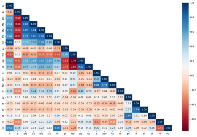
皮尔逊相关系数的热图如图所示。 1,它显示了数据集中的变量对之间的线性相关性。系数在1.0和1.0之间,1.0是强大的负相关性,1.0是强烈的正相关,而0几乎没有线性相关。高达0.84的强正相关和强大的负相关性降至-0.66是显着的。这些值的基本含义是,某些特征对高度相关,这可能会影响模型预测以及结果解释。

输入和输出参数之间的相关性。
图 2代表两组数据集,VC和VS的内核密度估计器密度(KDE)的直方图与许多归一化性状的密度进行比较。直方图中值的频率分布可视化,但KDE绘制了描绘给定数据集的每个概率密度函数的平滑线和曲线。归一化值是在X轴上采用的,这些值的频率的恒定密度在y轴上取。每个子图表示一个功能。显示VC的数据集以红色曲线显示,并且显示的数据集以绿色曲线显示。已经发现,VC数据的浓度在归一化值的尺度的低侧很重,另一方面,VS数据的浓度在整个尺度上或多或少地均匀下降。当输入的分布基本上类似于VU的分布时,输出可能表明更大的统计依赖性或灵敏度,这可能表明对输出变化的贡献更大。另一方面,低相关性或影响是由输入和VU的形状,扩散或峰位置之间的巨大差异指示。BF1,PL,FV和VR等特征的形状分布与VU截然不同,表明较低的统计依赖性和可能对输出的重要性有限。其他输入(如AC,FY和PP)是中等相似的,这意味着存在某种或条件效应。该图显示了诸如VP,DF和LF等输入分布的清晰度和偏差,这些输入的影响很小,或者可能以更复杂的方式与VU相互作用。这样的可视化对每个数据集的行为和特性的特殊性有益于区分和表征,并为进一步分析其特征提供了数值基础。

每个功能之间的关系。
图 3说明了用于该项目的系统研究方法。最初,影响剪切行为的数据是从各种研究中收集的。后来,为了开发模型,这些数据用于开发,训练和测试模型。首先,清理数据,然后将其分为一个培训数据集,该数据集具有80%的数据,以及一个具有20%数据的测试数据集。该模型使用XGB作为数学方法的主要预测方法和方法,包括果阿,LSA和SHO设置超参数。K折的交叉验证提高了模型的可靠性,因为它分配了每组数据集用于训练和测试模型。当检测到高误差时,进行了进一步的优化。随后,将模型的精度与经验模型进行了比较,以验证模型的性能在达到令人满意的水平后。最后,将SHAP应用于解释模型并确定剪切行为预测中每个参数的重要性。这种系统的方法产生了一个有效且易于解释的模型,可以预测UHPC梁的剪切强度。

当前研究的研究方法。
软计算技术
极端梯度提升(XGB)
XGB是基于梯度提升框架的广泛采用的集合模型。它用于借助几个决策树来预测输出56,,,,57,,,,58。这些树木被分析为弱学习树,并且在即将到来的树木中纠正了所产生的错误,使它们成为强大的学习树。该过程涉及减少损失函数,预测弱学习者,并添加额外的损失函数以最大程度地减少误差。学习率,树的深度和正则化技术的使用有助于很好地优化性能。使用等式计算损失函数(1) 和 (2)。
$$ {\ MATHCAL {l}}}^{t} = \ sum_ {i = 1}^{n} l \ left({y} _ {i,}i}^{\ left(t-1 \ right)}+{f} _ {t} \ left({x} _ {i,} \ right)\ right)\ right)+\ omega\ left({f} _ {t} \ right)$$
(1)
$$ \ omega \ left(f \ right)= \ gamma t+\ frac {1} {2} {2} \ lambda {\ vert \ omega \ emega \ vert}^{2} $ $
(2)
在哪里\({\ Mathcal {l}}}^{t} \)=损失功能,\({y} _ {i,} \ wideHat {y} = \)标记的数据和预测数据,\({f} _ {t} \)= t的模型Th树,tâ=迭代索引,t =树叶总数,\(\ lambda \)和\(\ gamma \)是惩罚系数,\(\ omega \)是每个叶子分数的矢量。
巨型武装算法(果阿)
Giant Armadillo算法(GOA)是一种最近开发的元启发式算法,其灵感来自于狩猎行为,以巨大的武术52。元启发式算法是使用两个阶段对数学建模的。首先,对空间的探索集中在于巨型武装行动寻找白蚁丘。最后一步是基于空间的开发。它重点介绍了巨型舰队的挖掘策略,以攻击白蚁的土墩。使用等式初始化决策变量值。(3)根据等式中提供的矩阵空间表示中的巨型武器刀的起始位置(4)。尽管有效,但是当猎物靠近一个密封(领导者)而远离其他密封件时,MLPA仍缺乏准确性。为了解决这一缺陷,使用加权领导者的猎物分配(WLPA),从而将指定的领导者分配为重量取决于其靠近猎物的权重,称为w_i。猎物的预期位置可能表示为
$$ {x} _ {i,d} = l {b} _ {d}+r \ cdot \ left(u {b} _ {d} _ {d} -l {b} _ {d} _ {d} \ right)$$
(3)
$ x = \ left [{\ begin {array} {*{20} c} {x__ {1}}} \\ \ \ \ \ \ \ \ \ \ \ \ \ {\ begin {array} {*{20} {20} c}} \\ {x_ {n}} \\ \ \ end {array}}}}} \\ end {array}}}}}} \ \ \ \ \ \ \ \ \ \ \ \ \ \ \ \ \ \ \ \ \右] _ {n \ times m} = \ weft {n \ times m}\ ldots&{x_ {1,d}}&\ ldots&{x_ {1,m}}} \ \ \ \ \ \ \ \ \ \ \ vdots&{\ ddots}&{\ Mathinner\ rish4pt \ hbox {。} \ mKern2mu \ rish7pt \ hbox {。} \ mkern1mu}}}&\ vdots \\ {x_ {x_ {i,1}}}}}}&\ ldots&\ ldots&{x__&{\ Mathinner {\ Mkern2mu \ rish1pt \ hbox {。} \ Mkern2mu \ rish4pt \ hbox {。} \ Mkern2mu \ rish7pt \ hbox \ hbox {。{x_ {n,1}}&\ ldots&{x_ {x_ {n,d}}&\ ldots&{x_ {x_ {n \ times m}}} \ \ \ \ \ end {array}}}}} \ right] _ {
(4)
x表示果阿的种群矩阵,x我是我Th果阿成员的位置状态。xID是dTh搜索空间维度,n是巨型腋窝的总数,m是变量的数量,r表示间隔[0,1]中的随机数空间,lbd和ubd指示D的下部和上限Th分别可变。等式(5)评估由巨型舰队位置提出的每个候选解决方案的目标函数值。$ f = {\ left [\ begin {array} {c} {f} _ {1} \\ \ \ \ \ \ \ \ \\ \ \ \ \ \ \ \ \ begin {array} {c} {f} {f} _ {i}
{f} _ {n} \ end {array} \ end {array} \ right]} _ {n \ times 1} = {\ left [\ left [\ begin {arnay} {c} f \ left(\ begin {array} {c} f \ left({x} _ {i} \右)
(5)
在这里,F和F我是目标函数的向量和I的目标函数Th果阿成员。等式中显示了每个成员的此类位置集
6)。新位置被随机更新为从一组候选白蚁丘集中的白蚁丘之一,并使用等式进行了攻击(7)。
$ t t {m} _ {i} = \ left \ {{x} _ {k}:{f} _ {k} <f {} _ {i}和k \ ne i}和k \ ne i \ right \ rigr\ dots,n \ right \} $$
(6)
在这里,TM我是我的位置Th巨型舰队,用于一套候选白蚁丘,Xk是总人口成员的目标函数价值比ITh巨型武术8)$$ {x} _ {i,j}^{p1} = {x} _ {i,j}+r {} _ {i,j} \ cdot \ left(stm {} _ {} _ {i,j} - {i,j} -
(7)
$ x_ {i} = \ left \ {{\ begin {array} {*{20} c} {x_ {x_ {i}^{{p1}},}&{f_ {f_ {i}
\ end {array}}} \ right。$$
(8)
在这里,STM我是被收养的白蚁丘Th巨人舰队,Stm我,j是它的J。Th方面,\({x} _ {i}^{p1} \)是为I计算的更新位置Th巨型舰队。提议的果阿的进攻阶段,\({x} _ {i,j}^{p1} \)是它的J。Th方面,\({f} _ {i}^{p1} \)是其目标函数值,\(r {} _ {i,j} \)是间隔[0,1]的任意数字,I我,j是任意选择的数字。
在剥削阶段,对巨型舰队在白蚁上打开土墩和猎物的挖掘作用进行了建模。这会导致巨大的员位置发生了很小的变化,这增加了算法在当地搜索空间中的剥削。因此,根据等式计算的新职位(9根据等式,会员的初始位置更改)(10),目标函数的值得到增强。
$$ {x} _ {i,j}^{p2} = {x} _ {i,j}+\ left(1-2 {r} _ {i,j} \ right)\ cdot \ cdot \ cdot \ frac {u {u {b}
(9)
$ x {} _ {i} = \ left \ {\ begin {array} {c} {c} \ begin {array} {cc} {x} {x} _ {i}^{p2}^{p2},&{f}f {} _ {i},\ end {arnay} \\ \ begin {array} {cc} {cc} {x} _ {i},&else \ end \ end {array} \ end} \ end {array} {array} \ right。$ $ $
(10)
这里,\({x} _ {i}^{p2} \)是为I计算的更新位置Th在拟建果阿的挖掘阶段,巨型舰队,\({x} _ {i,j}^{p2} \)是J。Th方面,\({f} _ {i}^{p2} \)是其优化的目标函数值,\({r} _ {i,j} \)是[0,1]间隔中的任意数字,t是总迭代。斑点鬣狗优化(SHO)
斑点的鬣狗优化(SHO)是一种自然风格的元神经化算法,从生活方式中绘制出,然后是斑点
53。鬣狗的独特行为是女性鬣狗是最主要的成员。此外,鬣狗的组合听起来与人笑相似,以调查食物来源。SHO算法的数学建模涉及包围猎物,狩猎猎物,攻击和搜索。SHO算法有效地在进一步迭代中找到最佳解决方案。如图所示,涉及的方程式11) 和 (12)表示遵循的不同步骤:
$$ {\ oferrightArrow {d}} _ {h} = \ left | \ offrightArrow {b} \ cdot {\ oftrightArrow {p}} _ {p} _ {p} \ left(x \ weles(x \ oright)
(11)
$ \ oftrightArrow {p} \ left(x+1 \ right)= {\ overrightArrow {p}} _ {p} \ left(x \ right) - \ offerrightArrow {e} \ cdot {\ cdot {\ costrightArow {\ costrightArow {
(12)
在哪里\({\ oftrightArrow {d}} _ {h} \)定义猎物和鬣狗之间的距离(请参阅等式 13),\(x \)指示更新的迭代,\(\ oftrightarrow {b} \)和\(\ oftrightarrow {e} \)是共同的向量,\({\ overrightArrow {p}} _ {p} \)指示猎物的位置向量,\(\ oftrightarrow {p} \)是斑点鬣狗的位置向量。
$$ \ oferrightArrow {b} = 2 \ cdot r {\ oftrightArrow {d}} _ {1} $$
$$ \ oferrightArrow {e} = 2 \ oftrightArrow {h} \ cdot r {\ costrightArrow {d}} _ {2} - \ costerrightArrow {h h} $$
$ \ oferrightArrow {h} = 5- \ left(itr \ right。*\ left(5/\ right.max \ left,ma {x} _ {\ text {itr}} $$
(13)
可以使用等式对狩猎行为进行建模(14)。
$$ {\ oftrightArrow {d}} _ {h} = \ left | \ offrightArrow {b} \ cdot {\ overrightArow {p offerrightArow {p}} _ {h} _ {h} - {\ costrightArrow {P}
$$ {\ oftrightArrow {p}} _ {k} = {\ oftrightArrow {p}} _ {h} - \ oftrightArrow {e} \ cdot {\ cdot {\ overrightArrow {d}}}} _ {h} $$
$$ {\ oferrightArrow {c}} _ {h} = {\ offrightArrow {p}} _ {k}+{\ oftrightArrow {p}} _ {k+1}+1}+dots+dots+dots+{\ dots+{\ offrient arterrightArrow {
(14)
在哪里\({\ oftrightarrow {p}} _ {h} \)代表第一个最斑点鬣狗的位置,\({\ oftrightArrow {p}} _ {k} \)代表其他斑点鬣狗的位置。\(n \)是由等式计算的斑点鬣狗的数量(15)。
$ n = {\ text {count}} _ {\ text {nos}} \ left({\ overrightArrow {p}} _ {h},{\ oftrightArrow {p}} _ {p}} _ {H+1},{,\ left({\ overrightArrow {p}} _ {h}+\ oftrightArrow {m} \ right)\ right)$$
(15)
在哪里\(\ oftrightarrow {m} \)是一个随机向量\(\左[0.5,1 \ right] \),NOS定义了解决方案的表示,并计算所有候选解决方案。还,\({\ oftrightArrow {c}} _ {h} \)代表一个或集群\(n \)最佳解决方案的数量。攻击是对等式进行的(16)。
$$ \ oferrightArrow {p} \ left(x+1 \ right)= \ frac {{\ oftrightArrow {c}} _ {h}}} {n} $$
(16)
在哪里\(\ oftrightarrow {p} \ left(x+1 \ right)\)\)保存最佳解决方案并更新搜索代理的位置。
豹密封优化(LSA)
豹密封优化(LSA)是一种新型优化方法,灵感来自豹密封的觅食行为54。无论他们的饥饿程度如何,他们总是在寻找猎物时保持警惕。他们的行为表明他们通过为每个人分配一定的搜索范围来实践自我分布。海豹牛群成员发现猎物后,其他成员聚集在附近并发起统一的罢工。LSO模型具有三个顺序阶段:(i)猎物搜索,(ii)猎物包围和(iii)猎物攻击。以下一节以数字说明了狮子密封的捕食优势。
豹密封的位置向量在每个周期中移动过程中,表示\(\ xi \),保持正确的维护。i的初始点Th循环 (\({\ oftrightarrow {x}} _ {init}^{j} \)\))事先已知,因为它表示(i 1)中螺旋的终点Th迭代,也可以用\({\ oftrightarrow {x}} _ {\ xi}^{i-1} \)。\({\ oftrightarrow {x}} _ {1}^{i} \)和\({\ oftrightarrow {x}} _ {\ xi}^{i} \)表示当前和I的初始点和终点Th分别迭代。在每个搜索阶段迭代中,\(\ xi \)漫游豹密封的位置向量表示为\({\ oftrightArrow {x}} _ {p}^{i} \ forall p \ in \ in \ {\ text {1,2},3,\ dots,\ xi \ xi \} \)目标函数的价值是\({f(\ oftrightArrow {x}} _ {p}^{i})\ forall p \ in \ in \ {\ text {1,2},3,\ dots,\ dots,\ xi \} \)。这\(\ xi \)i的位置向量Th印章的迭代\({l} _ {m} \)由等式计算17)。$ $ {\ oferrightArrow {x}} _ {\ alpha}^{i}({l} _ {m})| \ forall \ alpha \ in \ text {1,2},3,3,\ dots,\ dots,\ dot
-1 = {\ oftrightArrow {d}}^{i}({l} _ {m})。{\ overrightArrow {x}} _ {\ xi}^{i} {l} {l} _ {m} $$
(17)
在哪里\({\ oftrightArrow {x}} _ {\ alpha}^{i}({l} _ {m})\)\)\)是新的\(\阿尔法\)的位置\({l} _ {m} \)在决赛中Th迭代和\({\ oftrightArrow {d}}}^{i}({l} _ {m})\)\)\)是豹密封及其猎物之间的距离。第二阶段是用于猎物的包围,其中搜索剂遏制了猎物并找到最佳解决方案。
该阶段的主要障碍是猎物的位置尚未预先知道,因此需要事先分配猎物的位置。单领导者猎物分配(SLPA)是猎物分配的最简单方法。基于SLPA,如等式所示,证明了猎物的位置18)。
$$ {\ oftrightArrow {x}} _ {prey} =位置\ left [\ begin {arnay} {c} argmax \ _validation [f \ left({l} _ {l} _ {m} _ {m} \ right)]
(18)
s是搜索代理集和\(f \ left({l} _ {m} \ right)\)\是LSA算法的健身函数。另一种方法是多领导者猎物分配(MLPA)。如果Z维空间中有K领导者,则\({i}^{th} \)领导者可以表示为:\ \({\ oftrightArrow {x}} _ {i} = [{x} _ {1i},{x} _ {2i},{x} _ {3i} \ dots ..。猎物的预测位置可以由等式代表(19)。
$$ {\ oftrightArrow {x}} _ {prey} = \ frac {1} {k} {k} \ left(\ genfrac {} {} {} {0pt} {0pt} {} {\ begin {arnay} {array} {array} {c} {c} {c} {\ sum} _ {i = 1}^{k} {x} _ {1i} \\ {\ sum} _ {i = 1}^{k} {k} {x} {x} _ {2i}\\\\\\\\\\\\\\\\\\\\\\\\\\\\\\\\\\\\\\\\\\\\\\\\\\\\\\\\\\\\\\\\乱H{\ sum} _ {i = 1}^{k} {x} _ {zi} \ end {array}}} \ right)$$
(19)
如果猎物的位置非常靠近领导者密封,并且离其他密封很远,MLPA虽然有效,却不准确。To rectify this deficiency, Weighted Leaders Prey Allocation (WLPA) is used, whereby designated leaders are allocated a weight contingent upon their proximity to prey, denoted by an assigned weight w_i.The anticipated location of the prey might be denoted by Eq. (20)。
$${\overrightarrow{X}}_{prey}=\frac{1}{{\sum }_{m=1}^{k}W({L}_{m})}\left(\genfrac{}{}{0pt}{}{\begin{array}{c}{\sum }_{m=1}^{k}W\left({L}_{m}\right).{x}_{1m}\\ {\sum }_{m=1}^{k}W\left({L}_{m}\right).{x}_{2m}\\ \dots \end{array}}{\begin{array}{c}\dots \\ \dots \\ {\sum }_{m=1}^{k}W\left({L}_{m}\right).{x}_{zm}\end{array}}\right)$$
(20)
When the prey is encircled and cannot move further, the agents come nearer the prey and eventually capture it.The distance between the agent and the prey (\({\overrightarrow{D}}_{{L}_{m}}^{i})\)in this phase is calculated by Eq. (21)。
$${\overrightarrow{D}}_{{L}_{m}}^{i}=\left|{\overrightarrow{X}}_{prey}^{i}-{\overrightarrow{X}}_{{L}_{m}}^{i}\right|$$
(21)
Modelling and hyperparameter tuning
K-fold cross-validation is a reliable and extensively used technique to reduce overfitting problems.The procedure starts when the subdivided training data uses the remaining subgroup data for testing and the K−1 data of the whole K fold59。Every iteration of this algorithm uses the validation data once.The final model’s performance is defined as the mean performance across all k folds in testing and training.If an accepted model performs well during training but poorly on unknown data, it is deemed overfitted.For this study, the dataset was first divided into 80:20 training and evaluation sets.It had 80% of the training data and 20% of the assessment data, which were not repeated in the training set;tenfold cross-validation that used 80% of the total data for training may be a better option to avoid bias in the test set.There were ten sets in total: nine of them were employed for training the dataset, and the tenth set was employed for testing the dataset.The modelling was considered to be valid after the total performance in every fold was calculated.It turned out that each fold had different data in the testing set.However, to enhance the models’ performance before the training set, the hyperparameters needed to be tuned.In other words, hyperparameters are the variables that exist outside the model and are used by the algorithm to fine tune the performance of the model in question.This leads to the efficient tuning of hyperparameters and therefore an increase in the model’s accuracy.XGB adjusted parameters, including learning rate, max_depth, and n_estimators, to enhance the model’s efficiency and accuracy.The GOA, SHA, and LSA are metaheuristic algorithms that optimize the hyperparameters of the XGB algorithm.Defining the MHA parameters and establishing the bounds before optimization.For MHA, the parameters specified are population (n_pop), maximum iterations (max_iter), and number of hyperparameters (dim).Subsequently, to ascertain a standard hyperparameter value, optimization is performed to minimize the cost function, namely the Root Mean Square Error (RMSE).Both approaches possess the following parameters: dim = 3, cost_func = RMSE, max_iter = 100, and n_pop = 50.桌子2presents the comprehensive hyperparameter results.Table 2 Hyperparameter result of the applied hybrid model.
The assessment of the model’s performance in training and testing sets is crucial prior to the deployment of the model.
This assessment is possible using datasets with performance indicators that still need to be made evident.By advancing the model’s generalization, each metric strengthens the model’s reliability.Equations (22–27) present the six statistical parameters that are employed in this inquiry.To improve the performance evaluation, several statistical indicators may be used, including R2, variance account factor (VAF), mean absolute error (MAE), Willmott’s index of agreement (WI), Root Mean Square Error (RMSE), and a20 index.
$${R}^{2}=\frac{\sum_{i=1}^{N}{\left({y}_{i}-{y}_{mean}\right)}^{2}-\sum_{i=1}^{N}{{(y}_{i}-{\widehat{y}}_{i})}^{2}}{\sum_{i=1}^{N}{\left({y}_{i}-{y}_{mean}\right)}^{2}}$$
(22)
$$\text{RMSE}=\sqrt{\frac{1}{N}\sum_{i=1}^{N}{{(y}_{i}-{\widehat{y}}_{i})}^{2}}$$
(23)
$$MAE=\frac{1}{N}\sum_{i=1}^{N}|{\widehat{y}}_{i}-{y}_{i}|$$
(24)
$$WI=1-\left[\frac{\sum_{i=1}^{N}{{(y}_{i}-{\widehat{y}}_{i})}^{2}}{{\sum_{i=1}^{N}\left\{|{\widehat{y}}_{n}-{y}_{mean}|+|{y}_{n}-{y}_{mean}|\right\}}^{2}}\right]$$
(25)
$$VAF\left( \% \right) = \left( {1 - \frac{{VAR\left( {y_{i} - \hat{y}_{i} } \right)}}{{VAR(y_{i} )}}} \right) \times 100$$
(26)
$$a20 index=\frac{n20}{n}$$
(27)
where, y我 = iThmeasured value,\({\widehat{{\varvec{y}}}}_{{\varvec{i}}}\)= iThpredicted value, y意思是 = mean of the measured value, N = total number of readings, R2 = coefficient of determination, RMSE = Root Mean Squared Error, MAE = Mean absolute error, WI = Willmott’s Index of Agreement, VAF = Variance Account Factor.
Results and discussion
Performance comparison of the employed model
The performance of the hybrid machine learning models—GOA-XGB, SHO-XGB, and LSA-XGB for predicting the shear strength of UHPC beams is presented in Tables3和4。This analysis provides both the training and testing phases of models.It gives an overall assessment of the prediction performance, error, and reliability of each model, which are paramount in civil engineering applications.Starting with the R2score, which measures how well each model explains the variance in the data, all models exhibit exceptionally high R2values during the training phase: GOA-XGB gets 0.9941, SHO-XGB gets 0.9943, and LSA-XGB gets a slightly lower score of 0.9912.These values indicate that each model accounts for about 99% of the variability of the shear strength data and thus provides a good fit to the training dataset.
Nonetheless, the 0.001 difference in R2scores of the LSA-XGB may imply that it is less likely to over-fit compared to the training phase, since tested again during the testing phase.In the testing phase, coefficients of determination, R2scores, decrease a bit, which is normal because models work with unknown data.Despite this decrease, the R2values remain high: The R2score of GOA-XGB is 0.9570, SHO-XGB is 0.9594, and the best R2score is achieved by LSA-XGB with 0.9802.This high accuracy can be attributed to the LSA feature to efficiently explore the hyperparameter space of the XGB model without exaggerating the training data54。This shows that LSA-XGB outperforms the other models in terms of generalization, especially because the model complexity is well-balanced with the data fitting capability.The result showed enhanced prediction capacity compared to previous existing research works14。The testing phase results indicate that LSA-XGB can be the most suitable model for practical use when it is crucial to predict the results of new data.Other evaluation criteria that show the accuracy of each model are the RMSE and MAE.In the training phase, the RMSE values are very low for GOA-XGB at 0.0104, SHO-XGB at 0.0102, and LSA-XGB at 0.0127.This pattern is consistent with the MAE values: The results show that GOA-XGB has the lowest error at 0.0069, followed by SHO-XGB at 0.0071, while LSA-XGB has a slightly higher error at 0.0089.These low error values are able to substantiate the fact that the models yield near-correct predictions in the training phase.In the testing phase, RMSE and MAE values increase slightly, which is the expected drop in performance on new data.GOA-XGB has an RMSE of 0.0318 and an MAE of 0.0210;SHO-XGB has an RMSE of 0.0309 and an MAE of 0.0212;and LSA-XGB has slightly better results with an RMSE of 0.0306 and an MAE of 0.0208.The results of the testing phase indicate that LSA-XGB has a more appropriate level of generalization because the corresponding RMSE and MAE values are lower.
Further supporting the models’ credibility and stability are the A20 index, W(I), VAF, and U95 measures.The a20 index, which quantifies the proportion of predictions that are within a 20% range, is very small in the training set at about 0.0008 and slightly higher in testing.Such a low a20 index shows that the models’ predictions are very near reality and are quite precise.The WI values, which are near 1.0 for both training (0.9985) and testing (0.9886) sets, showed that the models have good conformity with the observed values and that the models are consistent.VAF values are above 95% for both phases, indicating that the models are good at reproducing almost all the data variability, with training VAFs peaking at 99.4%.The low U95 values in both phases suggest that there is little variability in the prediction, which is beneficial for the application of the models.Therefore, the high R2values, low RMSE and MAE, high WI and VAF, and low U95 indicate that GOA-XGB, SHO-XGB, and LSA-XGB are very efficient in predicting the shear strength of UHPC beams.Even in the training phase, GOA-XGB and SHO-XGB have a high accuracy, but in the testing phase, LSA-XGB has a higher R2score, fewer errors, and thus is the ideal model for use in practice.These findings demonstrate the effectiveness of hybrid machine learning models in improving structural prediction reliability in civil engineering, offering dependable tools to enhance UHPC design, material efficiency, and safety.
Further, Figs. 4和5illustrate scatter charts of the measured shear strength (Vu, test) as well as the shear strength predicted by the ML models (Vu, pred).In these plots, the horizontal axis represents the test values, and the vertical pace shows the Vu and pred values.The greater the accordance of the dots with the black diagonal line that corresponds to y = x, the better the correspondence of the ML model to the distribution of the effect of input factors on the predicted shear strength.Notably, when comparing Figs. 4和5, most predicted points from all ML models for the test dataset closely align with the y = x line, as all models were optimized on the training dataset using different techniques.This means that for all the ML models generated, we can confirm that, indeed, they fit the data.In Fig. 4, which presents the results for the training datasets, the predicted strength values are closely aligned with the actual strength values across all three models.This strong correlation is visually apparent through the tight clustering of data points around the best-fit line, indicating a high level of predictive accuracy.For the GOA-XGB model, represented by red data points, most predicted values closely follow the actual strength values, with minimal deviation.Only a small number of points stray from the best-fit line, suggesting that the model is well-tuned to the training data.

Actual vs. Predicted plot in training datasets.

Actual vs. Predicted plot in testing datasets.
The SHO-XGB model, shown in yellow, also displays a strong fit, although some deviations are observed at higher strength values.Despite these minor variances, the majority of data points remain close to the best-fit line, indicating that the SHO-XGB model performs reliably on the training data.Meanwhile, the LSA-XGB model, represented by blue points, demonstrates the highest level of accuracy among the three models.The predicted values almost perfectly follow the actual strength values, with very few points deviating from the best-fit line, showing that this model has been finely tuned to the characteristics of the training data.In Fig. 5, which illustrates the performance of these models on the testing datasets, the overall trends remain consistent.However, there is a slight increase in variability when compared to the training data.The GOA-XGB model, again represented by red points, shows a strong correlation between predicted and actual strength values.However, a few more deviations are noticeable in the higher strength ranges, indicating a slightly reduced accuracy when applied to unseen data.Nevertheless, the majority of points still align closely with the best-fit line, demonstrating the model’s strong predictive capability even on the testing set.
For the SHO-XGB model, displayed in yellow, the predicted values continue to follow the actual strength values closely, though the variance in mid-range strength values is more pronounced compared to the training set.This suggests that while the model generalizes well to unseen data, it may show a slight decline in performance at certain strength ranges.However, it still maintains a reasonably strong overall correlation, as most data points cluster near the best-fit line.The LSA-XGB model, represented by blue dots, again shows the best performance with the least error between the predicted and actual values, including the testing set.The majority of the predicted values are still quite accurate in terms of the actual strength values, and the points are clustered around the regression line.This agreement across both the training and testing sets shows that the LSA-XGB model has excellent out-of-sample prediction ability and is ideal for usage in both the training and testing datasets.In general, the comparison between Figs. 4和5shows that the XGB models are quite reliable.Although the accuracy is slightly lower when the model is applied to the test data, the models, especially LSA-XGB, remain quite effective.The figures taken all together underscore the models’ capacity for identifying the structure of the data in the training set and then reproducing that performance in the testing set – a key factor for successful use in practical applications.The LSA-XGB model, for instance, demonstrates a high level of stability in the obtained accuracy across both datasets, thus being the most suitable model for strength values forecasting in this analysis.
Model evaluation and validation techniques
Figure 6shows the RMSE convergence of the three models used in this study, namely GOA-XGB, SHO-XGB, and LSA-XGB.The first axis on the graph is the number of iterations, while the second one is the RMSE values.The graph gives information on how each model takes to converge and obtain the minimum error that it can perform during training.The GOA-XGB model, depicted by the red line, has the fastest rate of convergence to an RMSE of about 74 in a few iterations.The sharp decrease in RMSE indicates that the model quickly learns and adjusts its predictions during the initial stages of training, finding the optimal solution efficiently.The SHO-XGB model is shown in the blue line, and it is observed that it has a higher RMSE at the beginning of the iterations than the other models, but it gradually reduces after some iterations.However, in the final analysis, the RMSE is approximately 76, which shows that the model provides a slightly less precise solution than the GOA-XGB and LSA-XGB.The LSA-XGB model, shown in green, also exhibits a similar convergence trend to the GOA-XGB model but with a slightly higher initial RMSE.Following a sharp fall in RMSE, the LSA-XGB model attains the minimum error of about 73, suggesting that it is the most efficient of the three models in terms of this metric.

Convergence curve of all employed model.
The convergence differences between GOA-XGB, SHO-XGB, and LSA-XGB are because the former two models have a more efficient exploration–exploitation strategy.The GOA-XGB quickly decreased the RMSE by presetting on good solutions at the beginning of the process, which reduces the convergence time, albeit slightly reducing the final solution’s accuracy52,,,,60。SHO-XGB is a very slow learning algorithm, which tries to avoid RMSE minimum’s pitfalls of getting caught up in local minima and thus has a slightly higher RMSE53,,,,61。LSA-XGB can achieve both the highest exploration and the highest refinement, the fastest convergence and the lowest RMSE, thus being the most accurate of the three54。
In summary, Fig. 6shows that all three models can converge, but the LSA-XGB model is the most efficient in terms of RMSE, followed by the GOA-XGB model.The SHO-XGB model, although still effective, exhibits a higher error value, indicating that there is potential for further improvement.From the above convergence behaviour comparison, it is now clear that different models have unique efficiency and accuracy while training.
Additional statistical analysis was carried out to confirm the robustness and generalizability of the used models.The bootstrap residual resampling result of the LSA-XGB model, as shown in Fig. 7indicates a good fit between the predicted and true value of shear strength with a small 95 percent prediction interval.This suggests that the model is quite stable and substrata by biased with resampling.The histogram of the residuals in Fig. 8shows that they are normally distributed around zero, indicating that the errors are random and that the model is not too seriously overfitted.

Bootstrap residual resampling.

Model residual error of the best model.
Lastly, Fig. 9indicates the tenfold cross-validation of GOA-XGB, SHO-XGB, and LSA-XGB.Both LSA-XGB and the other methods have high values of R2in all folds, showing that they have good generalization performance.These tests support the reliability, accuracy, and resilience of the intended models to unexpected data division and random resampling.

Cross validation of employed models in tenfold.
Data visualization
Figure 10presents the Regression Error Characteristic (REC) curves for the GOA-XGB, SHO-XGB, and LSA-XGB models on both training and testing datasets.These curves provide a visual comparison of the accuracy of each model as a function of normalized absolute deviation.The x-axis shows the normalized absolute deviation, while the y-axis represents accuracy.The Area Under the Curve (AUC) is included as a measure of the overall performance for each model.In Fig. 10a, which depicts the performance on the training dataset, the LSA-XGB model (green curve) demonstrates superior performance with the highest AUC of 0.905, indicating that this model has the best accuracy for predicting training data.The SHO-XGB model (blue curve) follows with an AUC of 0.885, showing good accuracy but falling slightly short of LSA-XGB.The GOA-XGB model (red curve) has an AUC of 0.868, making it the least accurate of the three on the training set but still within acceptable performance limits.

Regression Error Characteristics (REC) Curve (一个) Training set (b) Testing Set.In Fig.Â
10b, the REC curves for the testing dataset reveal a similar trend, although the AUC values are slightly lower across all models.The LSA-XGB model remains the most accurate with an AUC of 0.819, followed closely by the SHO-XGB model with an AUC of 0.812.The GOA-XGB model, with an AUC of 0.815, also performs well, though all models show a small decrease in accuracy when applied to the testing data compared to the training data.The AUC differences stem from the fact that each model uses a different optimization approach.LSA-XGB outperforms all other models in terms of AUC because it finds a golden path in exploration and focused refinement, whereby it avoids many errors and can learn well from testing data.SHO-XGB has a wider scope but is not as precise when it comes to tuning, hence a slightly lower accuracy.GOA-XGB has a high convergence rate, which is good, but at the cost of the final accuracy, resulting in the lowest AUC.Therefore, LSA-XGB is the most reliable for accurate predictions with minimal deviation due to the balanced approach.The REC curves clearly illustrate the comparative effectiveness of each model in reducing prediction errors.A higher AUC indicates better overall performance, with the LSA-XGB model consistently demonstrating the best results on both training and testing datasets.These results provide strong evidence that the LSA-XGB model is the most reliable for making accurate predictions with minimal deviation.
Model explainability
Explaining how a machine learning model arrives at its predictions is essential for interpreting results, especially in complex models.SHAP provides a robust framework for assessing the contribution of each feature to the model’s output.Figures 8,,,,9, 和10collectively offer a deep dive into model explainability by utilizing SHAP values to illustrate the impact of individual features on the predictions.Figure 8displays the Mean Absolute SHAP Value Plot, which ranks the features based on their average SHAP values, showing their overall importance in influencing the model’s predictions.Here, the feature Ac stands out with the highest mean SHAP value of 193.27, indicating that it has the strongest effect on the model’s decisions.Other features like m (109.60) and pf (42.66) also play significant roles, but with a lesser impact compared to Ac.Features at the lower end of the scale, such as lf (2.61) and bf2 (1.94), have minimal influence on the model’s predictions.This ranking helps to identify the key drivers behind the model’s outputs and gives insight into which features are most influential.
Figure 11goes further by presenting a SHAP Summary Plot, which visualizes how each feature value affects the model’s predictions.The x-axis shows the SHAP values, and the color gradient (from blue to red) represents the range of feature values, where blue indicates lower values and red represents higher ones.For the feature Ac, a wide distribution of SHAP values is observed, showing both positive and negative impacts on the predictions.Higher values of Ac (red) generally push the predictions upwards, while lower values (blue) reduce the predictions.A similar pattern is observed for features like m and pf, where higher feature values are associated with increased SHAP values, indicating a positive influence on the predictions.This plot allows for a better understanding of not only which features are important but also how changes in feature values influence the model’s predictions.

Mean absolute SHAP value plot.
Figure 12takes a closer look at individual relationships between feature values and their SHAP values through a series of SHAP Scatter Plots.These scatter plots illustrate how each feature’s value directly affects its contribution to the model’s predictions.For instance, the feature Ac shows a strong positive correlation between higher values and increased SHAP values, suggesting that higher Ac values significantly boost the model’s predicted output.In contrast, features like pf demonstrate a negative correlation, where higher feature values lead to lower SHAP values and, consequently, lower predictions.Certain features, such as bf2 and df, exhibit smaller ranges of SHAP value changes, indicating that they play a less critical role in the overall prediction process.These plots provide detailed insights into the behavior of each feature and how its values influence the model’s output.In conclusion, Figs. 11,,,,12, 和13provide a thorough analysis of model explainability using SHAP values.Figure 11identifies the most important features, while Fig. 12illustrates how variations in feature values impact predictions.Finally, Fig. 13offers a closer look at the specific relationships between feature values and their contributions to the model’s output.Together, these figures provide a clear understanding of the model’s decision-making process and highlight which features are driving the predictions.

SHAP values.

Model explainability using SHAP values.
Besides the insights of the SHAP-based model, the Sobol global sensitivity analysis was also performed to measure the impact of input features on the model output.The total-order Sobol index indicates that Ac has a significant effect on the predicted shear strength (ST > 0.8), as shown in Fig. 14, and this confirms its dominant influence.m has a very small yet significant contribution, whereas the other features all have a very negligible influence.This homology of SHAP with Sobol outcomes increases the trust in the interpretation of feature importance and confirms that the decision-making process of the model is solid.

Sobol senstitivity analysis.
Comparison with existing empirical equations
Various existing codes are present to determine beams’ shear capacity, developed based on experiments, theories, and assumptions.However, the shear mechanism is complex as numerous parameters are involved.All of these parameters are hard to include in a single equation.The standard parameters for the shear capacity are section size, axial compressive strength, axial tensile strength, transverse reinforcement, longitudinal reinforcement, fiber factor, etc. Since the existing codes are based on some assumptions, getting precise results is difficult, making it necessary to modify the existing equation or use other advanced techniques.This research utilizes existing codes, such as Model MC2010, EN, AFGC-2013, and EN 1992-1-1, to predict shear and determine the shear capacity of UHPC beams.
Fib model code for concrete structures 2010 (Model MC2010)
For determining the shear capacity of FRC beams, Model MC201062has provided an equation as mentioned in Eq. (28)。This equation takes into account the contribution of the concrete from Eurocode 2. Parameters for his model include cylinder compressive strength, ultimate residual tensile strength, average tensile strength, average stress acting on the cross-section due to prestress and cross-sectional area.
$${\text{Vu}} = \left.{\left\{ {\frac{{0.18}}{{\gamma c}}k\left[ {100\rho s\left( {1 + 7.5\frac{{fFtuk}}{{fctk}}} \right)*fck} \right]^{{\frac{1}{3}}} + 0.15\sigma _{{cp}} } \right\}bwd} \right)$$
(28)
在哪里,
K is the size effect factor = 1+\(\sqrt{\frac{200}{d}}\) ≤ 2.
Here, d is the effective depth, Ïs is the longitudinal reinforcement ratio Astbwd Ïs\rho_sÏs​ is the longitudinal reinforcement ratio,fck​ is the compressive strength,fFtuk​ is the ultimate residual tensile strength, andfcuk​ is the concrete’s tensile strength (all in MPa).σCP​ represents prestress-induced stress,bwis the smallest width of the tension area, and Ï’c(safety factor) is taken as 1. IncorporatingfFtuk​ enhances the matrix with fiber benefits.French norm (AFGC-2013)
The French code AFGC-2013
63utilizes the truss model to determine the shear capacity of UHPC beams.The role of transverse reinforcement and fiber contribution is taken into consideration.The shear capacity is calculated by using Eq. (29)。
$$V = V_{c} + V_{s} + V_{f}$$
(29)
在哪里,vc-shear capacity contribution due to concrete matrix,vs—shear capacity contribution due to transverse reinforcement, andvf—shear capacity contribution due to fiber.
The three components are calculated using the following Eqs. (30–32)。
$$V_{c} = \frac{0.21}{{\Upsilon_{1} }}{\text{k}}_{2} {\text{f}}_{{\text{c}}}^{0.5} {\text{bd}}$$
(30)
where Ï’1is the safety factor, k2is the prestress coefficient, and b and d are the breath and effective depth, respectively.
$${\text{V}}_{{\text{s}}} = \frac{{A_{s} }}{s}zf_{y} cot\theta$$
(31)
在哪里一个sis the area of the stirrup, z is the distance between the top and bottom longitudinal reinforcement, s is the spacing of the stirrup, θ is the angle between the diagonal compression and the bottom and the beam axis taken as 45 degrees, fyis the yield strength of reinforcement.
$$V_{f} = \frac{{A_{b} \sigma_{Rd,f} }}{\tan \theta }$$
(32)
在哪里,一个bis the cross-section of the concrete matrix and σRd,fis the residual tensile strength.
European norm (EN 1992-1-1)
European norm (EN1992-1-1)64takes into account the shear capacity provided by the concrete matrix and stirrup.Shear capacity is calculated using Eqs. (33) 和 (34) as given in:-
$$\begin{gathered} V_{s} = V_{Rd,c} + V_{Rd,s} \hfill \\ V_{Rd,c} = C_{(Rd,c)} k(100\rho f_{c} k)^{(1/3)} b_{w} d \hfill \\ \end{gathered}$$
(33)
在哪里,cRd,c = 0.18/Ï’cwhere Ï’cis the partial safety factor,k = 1+\(\sqrt{\frac{200}{d}}\)where d is the effective depth,Ïis the reinforcement ratio
$$V_{Rd,s} = \frac{{A_{sw} f_{ywd} z}}{s}\cot \theta$$
(34)
在哪里,fckis the compressive strength of concrete (MPa),bw = the width of the cross-section,
一个SWis stirrup sectional area,z = internal lever height taken as 0.9d,sis be spacing of the stirrup, and我is the angle between the pressure bar and the longitudinal bar of the truss.FigureÂ
15presents a comparison of the efficiency of the shear capacity prediction models for UHPC beams, including Model Code 2010 (MC2010), French Norm (AFGC-2013), and European Norm (EN 1992-1-1) with the advanced machine learning-based model LSA-XGB.The conventional models, MC2010 and AFGC-2013, mainly overestimate the shear strength, which may result in unsafe design considerations due to over-estimation of the UHPC beams’ performance.This overestimation is evident as their data points are consistently above the ideal 1:1 ratio, which means that the predicted values would be equal to the actual measurements in the most accurate way.On the other hand, EN 1992-1-1 tends to overemphasize the shear capacity as a general rule, which may be a more safety-oriented approach that helps to avoid overloading structures and, at the same time, may produce designs that are not sufficiently effective in terms of using materials, thus unnecessarily increasing structural reinforcement costs unnecessarily.The LSA-XGB model, utilizing a sophisticated XGB algorithm, shows a remarkable alignment of predictions with actual data, indicated by the tight clustering of points around the 1:1 ratio.This high accuracy demonstrates the possibility of using more sophisticated models for the prediction of structural performance and reliability in the design of structures, especially those made of UHPC, which has special mechanical characteristics.These results underscore the need for more accurate, machine learning-based models to be incorporated into design codes for high-consequence structures.

Results from existing shear capacity prediction models and comparison with the current study.
桌子5shows the coefficient of regression (R2) and the theoretical to actual ratios of shear capacity.A high R2value nearly 1, for instance, 0.9802 in LSA-XGB, shows that high predictability and ratio values closer to 1 imply more accuracy.The LSA-XGB model gives the highest overall performance with an R2of 0.9802 and theoretical/actual ratio of 1.06, which suggests its predicted values are almost similar to the actual values.On the other hand, the other models, especially the European norm, have a large spread and lower accuracy, with the European norm model underpredicting, as evidenced by a ratio of 0.48.This analysis shows that there is a possibility of using machine learning techniques in structural engineering applications where accurate prediction of shear capacity is important, as compared to the use of traditional normative approaches.
The results of this study indicate that traditional models do not adequately capture the behaviour of UHPC beams, and future research should be directed toward refining or developing new shear capacity prediction methods that are more consistent with the unique structural characteristics of UHPC to ensure both safety and cost-effectiveness in design.
Since several parameters influence the shear behaviour of the UHPC beam, there is a critical issue in developing reliable and scalable modelling.To address this, an innovative GUI interface, as shown in Fig. 16,,,,is integrated using the best-adopted model in the study.GUI development aims to generalize the state-of-the-art implementation of developed models for engineers and researchers.This framework can be helpful in the estimation of the shear strength of beams using their data.Further, engineers can make quick decisions by understanding the parameters influencing shear strength in real time for reliable problem-solving.This study integrates numerous libraries, including Pickle and Tkinter of the Python programming language.This interface can be scalable by integrating application-based modules into structural software.

GUI for the prediction of shear strength of UHPC beam.
Conclusions
This research utilizes advanced machine learning techniques to predict the shear strength of UHPC beams.Combining XGB with metaheuristic algorithms, including GOA, SHO and LSA, this study has illustrated how high-level modelling techniques are used in predicting shear capacity.The vast collection of data has been a rich source for the benchmarking of these models and has been derived from various literature surveys containing a plethora of influential parameters.Additionally, this research evaluates the accuracy of existing codes.The following points summarize the key findings of this research:
-
(1)
The models demonstrated outstanding predictive performance;LSA-XGB had the highest testing R2(0.9802), followed by SHO-XGB (0.9594) and GOA-XGB (0.9570).With SHO-XGB at 0.9943, GOA-XGB at 0.9941, and LSA-XGB at 0.9912, all models obtained extremely high R2values during the training phase, demonstrating their ability to capture the variation in UHPC shear strength.(2)
-
The accuracy of the structural predictions was highlighted by the models’ low error rates across all investigations.
In testing, SHO-XGB achieved an RMSE of 0.0309 and MAE of 0.0212;GOA-XGB had an RMSE of 0.0318 and MAE of 0.0210;and LSA-XGB achieved the lowest errors, with an RMSE of 0.0306 and MAE of 0.0208.Additionally, throughout the simulation, all models had high VAF values above 95%, demonstrating the accuracy of the models’ predictions.
-
(3)
The LSA-XGB model had a better fit on the testing data with an R2of 0.9802.In comparison, existing empirical equations yielded lower R2values: 0.5930 for MC-2010, 0.8408 for AFGV-2013, and 0.5285 for EN 1992-1-1.These results show that the proposed LSA-XGB model is more accurate than the conventional methods used in the literature.
-
(4)
The comparison of various models, MC-2010, AFGC-2013, EN 1992-1-1, and the LSA-XGB hybrid model, revealed the following theoretical-to-actual prediction value ratios: 1.19, 1.12, 0.48, and 1.06, respectively.These results indicate that the LSA-XGB model provides predictions closer to actual values, outperforming traditional empirical equations.
-
(5)
The theoretical to actual prediction value ratios for the various model types—MC-2010, AFGC-2013, EN 1992-1-1, and LSA-XGB—were 1.19, 1.12, 0.48, and 1.06, respectively.This indicates that the hybrid prediction model that was developed outperformed empirical equations.
-
(6)
The application of GOA, SHO, and LSA algorithms in conjunction with XGB has successfully improved learning capabilities and optimized parameter tuning, demonstrating the potential of nature-inspired algorithms to tackle challenging engineering problems.
-
(7)
The findings indicate significant potential for using these models to improve the design, assessment, and management of UHPC structures, aligning with and potentially advancing current engineering codes and practices.The models provide a basis for revising existing design codes, which often do not fully account for the unique properties of UHPC.
-
(8)
Shapley Additive Explanations (SHAP) was employed, which improved the interpretability of employed ML models, vital for their broader acceptance and application in practical engineering scenarios.
-
(9)
Following model selection, a graphical user interface (GUI) was created for LSA-XGB to help engineers estimate UHPC shear strength.When designing UHPC beams, this GUI can be regarded as a useful, economical, and effective tool that enhances decision-making and aids in material optimization.
In summary, this study accurately predicted the shear strength of UHPC beams using an advanced machine learning algorithm.Understanding shear behavior and improving prediction model accuracy are still challenges.Despite the hybrid model’s high accuracy, there are still a number of areas that could be explored and improved.These include improving the incorporation of machine learning models into real-world engineering workflows, investigating the impact of extra variables, and tackling the constraints of diverse datasets.
Limitations of the current study and future research directions
The primary limitation of this study lies in the relatively smaller dataset that was used to develop prediction models.More reliable and useful insights might be obtained by enlarging the dataset to include samples from various geographical locations with different binding materials and material compositions.The dataset used was entirely sourced from existing experimental literature, which, while comprehensive, may limit the generalizability of the model to novel concrete mix designs, uncommon cross-sectional geometries, or structural elements subjected to dynamic or fatigue loading.Although the current study aimed at the development of accurate machine learning models to predict the shear strength of UHPC beams, it is desirable that in the future, this research be continued by including the measures of uncertainty and risk-informed models in an effort to aid more visibly in structural design-making.Additionally, this study employs a hybridized ensemble model, which is particularly good for smaller datasets.However, it becomes inefficient and computationally expensive for larger datasets.Future research can explore the application of deep neural network modelling to overcome this limitation.A significant limitation of the ML model is developing a predictive equation.Future research can focus on utilizing modelling techniques that are capable of establishing a robust correlation between input and output parameters.Likewise, it is frequently difficult to comprehend how features interact in complex models, which makes it more difficult to interpret their contributions.Moreover, while SHAP was employed for model interpretability due to its theoretical rigor and additive consistency, comparing it with other model explanation techniques, such as permutation feature importance and LIME, could further validate its selection.Interpretation based on domain knowledge representation is, therefore, crucial.Therefore, results from different explainable models are evident to corroborate a finding.Furthermore, with an increase in datasets, real-time approaches become essential to ensure efficient processing and prediction.Future research should focus on integrating real-time data processing techniques with ML models to enhance their scalability and practical applicability in dynamic environments.The future development should also include investigating higher-order feature selection and multicollinearity alleviation methods like Recursive Feature Elimination (RFE) and Variance Inflation Factor (VIF) analysis to achieve better robustness and interpretability of a model.
Data availability
当前研究期间和/或分析期间生成的数据集可从相应的作者根据合理的要求获得。
缩写
- UHPC:
-
Ultra-high-performance concrete
- ML:
-
机器学习
- NIA:
-
Nature-inspired algorithm
- XGB:
-
Extreme gradient boosting
- GOA:
-
Giant armadillo optimization
- SHO:
-
Spotted hyena optimization
- LSA:
-
Leopard seal optimization
- SHAP:
-
Shapley additive explanations
- 人工智能:
-
人工智能
- DT:
-
Decision trees
- SVM:
-
Support vector machines
- kNN:
-
K-nearest neighbours
- ANN:
-
Artificial neural networks
- KDE:
-
Kernel density estimator
- GBM:
-
Gradient boosting machine
- RFE:
-
Recursive feature eliminationr
- 2:Coefficient of regression
-
RMSE:
- Root mean squared error
-
MAE:
- Mean absolute error
-
VAF:
- Variance accounted for
-
GUI:
- Graphical user interface
-
VIF:
- Variance inflation factor
-
Ac:
- Area of concrete
-
m:
- Stirrup spacing
-
pf:
- Fiber pull-out force
-
bf1:
- Flange width 1
-
bf2:
- Flange width 2
-
tf1:
- Flange thickness 1
-
tf2:
- Flange thickness 2
-
Vu:
- Ultimate shear strength
-
h:
- Overall section height
-
b:
- Width of section
-
s:
- Stirrup spacing
-
pp:
- Prestressing strands
-
sp:
- Shear plane
-
psv:
- Prestressing steel volume
-
fsv:
- Shear strength of steel
-
fsy:
- Yield strength of steel
-
fc:
- Compressive strength of concrete
-
df:
- Diameter of fiber
-
lf:
- Length of fiber
-
参考
Ding, Y., Yu, K. & Li, M. A review on high-strength engineered cementitious composites (HS-ECC): Design, mechanical property and structural application.
Structures35 , 903–921 (2022).Google Scholar
一个 Akhnoukh, A. K. & Buckhalter, C. Ultra-high-performance concrete: Constituents, mechanical properties, applications and current challenges.
Case Stud.Constr.母校。 15, e00559 (2021).
de Larrard, F. & Sedran, T. Optimization of ultra-high-performance concrete by the use of a packing model.Cem.Concr.Res. 24, 997–1009 (1994).
Gong, J. et al.Utilization of fibers in ultra-high performance concrete: A review.Compos.B Eng. 241, 109995 (2022).
Wille, K., El-Tawil, S. & Naaman, A. E. Properties of strain hardening ultra high performance fiber reinforced concrete (UHP-FRC) under direct tensile loading.Cement Concr.Compos. 48, 53–66 (2014).
Yu, R., Spiesz, P. & Brouwers, H. J. H. Mix design and properties assessment of Ultra-High Performance Fibre Reinforced Concrete (UHPFRC).Cem.Concr.Res. 56, 29–39 (2014).
Fan, J., Shao, Y., Bandelt, M. J., Adams, M. P. & Ostertag, C. P. Sustainable reinforced concrete design: The role of ultra-high performance concrete (UHPC) in life-cycle structural performance and environmental impacts.工程。结构。 316, 118585 (2024).
Abbas, S., Nehdi, M. L. & Saleem, M. A. Ultra-high performance concrete: Mechanical performance, durability, sustainability and implementation challenges.Int.J. Concr.结构。母校。 10, 271–295 (2016).
Du, J. et al.New development of ultra-high-performance concrete (UHPC).Compos.B Eng. 224, 109220 (2021).
Xue, J. et al.Review of ultra-high performance concrete and its application in bridge engineering.Constr.建造。母校。 260, 119844 (2020).
Hung, C.-C., El-Tawil, S. & Chao, S.-H.A review of developments and challenges for UHPC in structural engineering: Behavior, analysis, and design.J. Struct.工程。 147, (2021).
Fan, D. et al.Intelligent design and manufacturing of ultra-high performance concrete (UHPC) – A review.Constr.建造。母校。 385, 131495 (2023).
Bajaber, M. A. & Hakeem, I. Y. UHPC evolution, development, and utilization in construction: A review.J. Market.Res. 10, 1058–1074 (2021).
Ye, M. et al.Prediction of shear strength in UHPC beams using machine learning-based models and SHAP interpretation.Constr.建造。母校。 408, 133752 (2023).
Yang, J., Doh, J.-H., Yan, K. & Zhang, X. Experimental investigation and prediction of shear capacity for UHPC beams.Case Stud.Constr.母校。 16, e01097 (2022).
Feng, W., Feng, H., Zhou, Z. & Shi, X. Analysis of the shear capacity of ultrahigh performance concrete beams based on the modified compression field theory.ADV。母校。科学。工程。 2021, (2021).
Qian, Y. et al.Prediction of ultra-high-performance concrete (UHPC) properties using gene expression programming (GEP).建筑物 14, 2675 (2024).
Bhusal, B. & Paudel, S. Comparative study of existing and revised codal provisions adopted in Nepal for analysis and design of Reinforced concrete structure.Int.J. Adv.工程。Manag. 6, 16–24 (2021).
Bhusal, B., Paudel, S., Tanapornraweekit, G., Maskey, P. N. & Tangtermsirikul, S. Seismic performance evaluation and strengthening of RC beam-column joints adopted in Nepal.在:Structures卷。57, p.105205 (Elsevier, 2023).
Mangalathu, S. & Jeon, J.-S.Classification of failure mode and prediction of shear strength for reinforced concrete beam-column joints using machine learning techniques.工程。结构。 160, 85–94 (2018).
Hamoda, A. et al.Experimental and numerical investigations of the shear performance of reinforced concrete deep beams strengthened with hybrid SHCC-mesh.Case Stud.Constr.母校。 21, e03495 (2024).
Paudel, S. & Bhusal, B. Investigation of modelling approaches for non-linear analysis of reinforced concrete frames.J. Eng.科学。技术。Rev. 14, (2021).
Jiang, H. et al.Experimental and numerical study on shear performance of externally prestressed precast UHPC segmental beams without stirrups.Structures 46, 1134–1153 (2022).
Huang, Y. & Yao, G. Shear strength of ultra-high-performance concrete beams without stirrups—A review based on a database.建筑物 14, 1212 (2024).
Cai, Z., Duan, X., Liu, L., Lu, Z. & Ye, J. Reinforced ultra-high performance concrete beam under flexure and shear: Experiment and theoretical model.Case Stud.Constr.母校。 20, e02647 (2024).
Abbood, I. S. Strut-and-tie model and its applications in reinforced concrete deep beams: A comprehensive review.Case Stud.Constr.母校。 19, e02643 (2023).
Zhang, X., Kho, W. & Li, B. Prediction of behavior of UHPC beams based on truss models.Structures 53, 642–651 (2023).
Abbas, A. A., Arna’Ot, F. H., Abid, S. R. & Özakça, M. Flexural behavior of ECC hollow beams incorporating different synthetic fibers.正面。结构。民用工程。 15, 399–411 (2021).
Chen, B., Zhou, J., Zhang, D., Sennah, K. & Nuti, C. Shear performances of reinforced ultra-high performance concrete short beams.工程。结构。 277, 115407 (2023).
Yousef, A. M., Tahwia, A. M. & Marami, N. A. Minimum shear reinforcement for ultra-high performance fiber reinforced concrete deep beams.Constr.建造。母校。 184, 177–185 (2018).
Jin, L.-Z., Chen, X., Fu, F., Deng, X.-F.& Qian, K. Shear strength of fibre-reinforced reactive powder concrete I-shaped beam without stirrups.Mag.Concr.Res. 72, 1112–1124 (2020).
Sahul, R. A review of: “Rheometry of pastes, suspensions, and granular materials: Applications in industry and environment â€.母校。Manuf.过程。 21, 934–934 (2006).
Zhang, Z. et al.Development of high-strength engineered cementitious composites using iron sand: Mechanical and shrinkage properties.J. Build.工程。 95, 110272 (2024).
Kumar, R. et al.Estimation of the compressive strength of ultrahigh performance concrete using machine learning models.Intell。系统。应用。 25, 200471 (2025).
Guo, K., Yang, Z., Yu, C.-H.& Buehler, M. J. Artificial intelligence and machine learning in design of mechanical materials.母校。Horiz. 8, 1153–1172 (2021).
Motie, M., Bemani, A. & Soltanmohammadi, R. On the estimation of phase behavior of CO2-based binary systems using ANFIS optimized by GA algorithm.in (2018).https://doi.org/10.3997/2214-4609.201803006。Ahmadi, S., Motie, M. & Soltanmohammadi, R. Proposing a modified mechanism for determination of hydrocarbons dynamic viscosity, using artificial neural network.
宠物。科学。技术。 38, 699–705 (2020).
Thai, H. T. Machine learning for structural engineering: A state-of-the-art review.Structures 38, 448–491 (2022).
Pandey, S., Paudel, S., Devkota, K., Kshetri, K. & Asteris, P. G. Machine learning unveils the complex nonlinearity of concrete materials’ uniaxial compressive strength.Int.J. Constr.Manag. https://doi.org/10.1080/15623599.2024.2345008(2024).
Paudel, S., Pudasaini, A., Shrestha, R. K. & Kharel, E. Compressive strength of concrete material using machine learning techniques.Cleaner Eng.技术。 15, 100661 (2023).
Rahman, J., Ahmed, K. S., Khan, N. I., Islam, K. & Mangalathu, S. Data-driven shear strength prediction of steel fiber reinforced concrete beams using machine learning approach.工程。结构。 233, 111743 (2021).
Feng, D.-C., Wang, W.-J., Mangalathu, S., Hu, G. & Wu, T. Implementing ensemble learning methods to predict the shear strength of RC deep beams with/without web reinforcements.工程。结构。 235, 111979 (2021).
Mangalathu, S., Shin, H., Choi, E. & Jeon, J.-S.Explainable machine learning models for punching shear strength estimation of flat slabs without transverse reinforcement.J. Build.工程。 39, 102300 (2021).
Xu, J.-G., Chen, S.-Z., Xu, W.-J.& Shen, Z.-S.Concrete-to-concrete interface shear strength prediction based on explainable extreme gradient boosting approach.Constr.建造。母校。 308, 125088 (2021).
Chhetri Sapkota, S., Dahal, D., Yadav, A., Dhakal, D. & Paudel, S. Analyzing the behavior of geopolymer concrete with different novel machine-learning algorithms.J. Struct.Des.Constr.Pract. 30, 04025027 (2025).
Feng, D.-C., Wang, W.-J., Mangalathu, S. & Taciroglu, E. Interpretable XGBoost-SHAP machine-learning model for shear strength prediction of squat RC walls.J. Struct.工程。 147, 04021173 (2021).
Solhmirzaei, R., Salehi, H., Kodur, V. & Naser, M. Z. Machine learning framework for predicting failure mode and shear capacity of ultra high performance concrete beams.工程。结构。 224, 111221 (2020).
Ni, X. & Duan, K. Machine learning-based models for shear strength prediction of UHPFRC beams.数学 10, 2918 (2022).
Kumar, R., Kumar, S., Rai, B. & Samui, P. Development of hybrid gradient boosting models for predicting the compressive strength of high-volume fly ash self-compacting concrete with silica fume.在:Structures卷。66, p.106850 (Elsevier, 2024).
Tipu, R. K., Batra, V., Pandya, K. S. & Panchal, V. R. Enhancing load capacity prediction of column using eReLU-activated BPNN model.在:Structures卷。58, p.105600. (Elsevier, 2023).
Tipu, R. K., Rathi, P., Pandya, K. S. & Panchal, V. R. Optimizing sustainable blended concrete mixes using deep learning and multi-objective optimization.科学。代表。 15, 1–26 (2025).
Alsayyed, O. et al.Giant armadillo optimization: A new bio-inspired metaheuristic algorithm for solving optimization problems.Biomimetics 8, 619 (2023).
Dhiman, G. & Kumar, V. Spotted hyena optimizer: A novel bio-inspired based metaheuristic technique for engineering applications.ADV。工程。软件。 114, 48–70 (2017).
Rabie, A. H., Mansour, N. A. & Saleh, A. I. Leopard seal optimization (LSO): A natural inspired meta-heuristic algorithm.社区。Nonlinear Sci.Numer.Simul. 125, 107338 (2023).
Zhang, L. et al.Experimental investigation on shear behavior of non-stirrup UHPC beams under larger shear span-depth ratios.建筑物 14, 1374 (2024).
Yan, Z., Chen, H., Dong, X., Zhou, K. & Xu, Z. Research on prediction of multi-class theft crimes by an optimized decomposition and fusion method based on XGBoost.Expert Syst.应用。 207, 117943 (2022).
Hoque, M. A., Shrestha, A., Sapkota, S. C., Ahmed, A. & Paudel, S. Prediction of autogenous shrinkage in ultra-high-performance concrete (UHPC) using hybridized machine learning.Asian J. Civil Eng. https://doi.org/10.1007/s42107-024-01212-8(2024).
Shrestha, A. & Sapkota, S. C. Hybrid machine learning model to predict the mechanical properties of ultra-high-performance concrete (UHPC) with experimental validation.Asian J. Civil Eng. https://doi.org/10.1007/s42107-024-01109-6(2024).
Lyngdoh, G. A., Zaki, M., Krishnan, N. M. A. & Das, S. Prediction of concrete strengths enabled by missing data imputation and interpretable machine learning.Cement Concr.Compos. 128, 104414 (2022).
Kyrou, G., Charilogis, V. & Tsoulos, I. G. Improving the giant-armadillo optimization method.分析 3, 225–240 (2024).
Ghafori, S. & Gharehchopogh, F. S. Advances in spotted hyena optimizer: A comprehensive survey.拱。计算。Methods Eng. 29, 1569–1590 (2022).
Kordina, K. R., Mancini, G., Schäfer, K., Schieβl, A. & Zilch, K.Fib Bulletin 54. Structural Concrete Textbook on Behaviour, Design and Performance Second Edition Volume 4。(fib. The International Federation for Structural Concrete, 2010).https://doi.org/10.35789/fib.BULL.0055。AFGC.
Ultra High Performance Fibre-Reinforced Concrete.建议。(2013)。
EN 1992-1-1: Eurocode 2: Design of Concrete Structures – Part 1: General Rules and Rules for Buildings。(1992).
资金
There is no funding for this research.
道德声明
竞争利益
作者没有宣称没有竞争利益。
Ethical approval
Not applicable.
Consent to participate
All authors agree to participate in the manuscript during revisions.
Consent to publish
All authors agree to the submission of manuscript.
附加信息
Publisher’s note
Springer Nature remains neutral with regard to jurisdictional claims in published maps and institutional affiliations.
补充信息
Rights and permissions
开放访问This article is licensed under a Creative Commons Attribution 4.0 International License, which permits use, sharing, adaptation, distribution and reproduction in any medium or format, as long as you give appropriate credit to the original author(s) and the source, provide a link to the Creative Commons licence, and indicate if changes were made.The images or other third party material in this article are included in the article’s Creative Commons licence, unless indicated otherwise in a credit line to the material.If material is not included in the article’s Creative Commons licence and your intended use is not permitted by statutory regulation or exceeds the permitted use, you will need to obtain permission directly from the copyright holder.To view a copy of this licence, visithttp://creativecommons.org/licenses/by/4.0/。Reprints and permissions
引用本文

Sapkota, S.C., Shrestha, A., Haq, M.
et al.Enhancing shear strength predictions of UHPC beams through hybrid machine learning approaches.Sci Rep15 , 28259 (2025).https://doi.org/10.1038/s41598-025-13444-y
已收到:
公认:
出版:
DOI:https://doi.org/10.1038/s41598-025-13444-y