Rosie：AI生成的多重免疫荧光从组织病理学图像染色

H＆E染色无处不在用于临床组织病理学，因为其可及性，可访问性和有效性可辨别临床相关特征。尽管H＆E很容易识别核和细胞质形态，但其效用在揭示与现代精确医学相关的更复杂的分子信息方面受到限制¹。病理学家可以单独鉴定出H＆E染色的各种细胞类型。但是，注释H＆E图像的计算方法仅区分一些广泛的细胞类别，例如内皮，上皮，基质和免疫细胞^{2，，，，3，，，，4}。这些方法对于检测肿瘤和识别基本结构特征是有价值的，但在揭示细胞微环境的详细方面有限，例如蛋白质表达谱，疾病特征，疾病特征或免疫细胞（如淋巴细胞）的特定认同。

相反，多质子免疫荧光（MIF）成像技术，例如通过索引（codex）和免疫组织化学（IHC）进行共检测，同时可以原位检测数十种蛋白质。这种能力允许探索富含组织的微环境，提供单独通过H＆E染色无法实现的见解^{5，，，，6，，，，7，，，，8}。但是，法典和类似MIF技术的应用受到高成本，耗时的协议以及在临床实验室中缺乏采用的限制，这使得它们不太适合常规使用⁹。

在这项工作中，我们介绍了Rosie（ro在计算机中的胸围我来自H＆e图像），基于H＆E染色的输入图像中硅米类染色的框架。我们在与H＆E和Codex共同染色的1,000多个组织样本的数据集上训练一个深度学习模型。该数据集包含近3000万个细胞，是迄今为止最大的数据集，并且显着超过了先前研究的规模，该研究通常集中于单个临床部位或有限数量的污渍的数据。我们的发现表明，所提出的方法可以仅凭H＆E染色就可以坚固地预测和空间解决数十种蛋白质。

我们验证了这些的生物准确性在有机硅生成中蛋白质表达通过在详细的细胞表型中使用，并发现组织结构（例如基质和上皮组织）。我们的方法可以鉴定免疫细胞亚型，包括单独使用H＆E染色无法发现的B细胞和T细胞亚型，从而提供了一种强大的工具来增强标准组织病理学实践的诊断和研究潜力。

培训组织病理学基础模型的最新进展^{10，，，，11，，，，12}已经证明，在适应下游任务（例如预测组织类型以及疾病诊断和预后）时，以无监督的方式进行了大型，多样化的组织学图像训练的模型。尽管基础模型可以在H＆E图像的分布中学习复杂的生物学特征，但仍需要对其他成像方式和分子信息进行明确训练，以适应诸如硅染色之类的生成方法。

先前预测H＆E免疫抑制剂的工作通常集中在小型配对或未配对的数据集上，并立即征服多个生物标志物。首先，VirtualMultiplexer是一种基于GAN的方法，用于预测6 plex IHC污渍¹³使用未配对的H＆E和IHC样品。使用未配对样本的局限性在于，预测的验证仅限于定性或视觉评估。几种方法已在配对（相邻切片）数据集上进行了培训，例如：Multi-V-stain¹⁴，它预测336个黑色素瘤样品上有10个Plex MIMC面板；Deepliif¹⁵它可以预测一个样品上的3 plex mihc；以及其他基于GAN的方法，用于预测单个或几种生物标志物^{16，，，，17，，，，18，，，，19，，，，20，，，，21，，，，22}预测脑组织上的两个IHC生物标志物。与配对样品相比，共同染色（或相同的切片）样品可以直接像素级对齐和从H＆E到免疫抑制剂的预测；为此，hemit（3-plex mihc）²³和VIHC（1-plex MIHC）都在共同染色的样本上训练，但也仅限于单个样本的评估²⁴。专注于使用4个共同染色样品预测转录组学面板（1000个基因）。特定于多重免疫荧光，7-UP²⁵使用一个小的7型式面板预测30多个生物标志物²⁶。使用自动荧光和DAPI通道来推断七个生物标志物。

我们的方法通过多种方式改善了以前的工作。首先，我们使用1300多个样品训练并评估最大的联合染色H＆E和免疫染色数据集。其次，尽管以前的数据集仅限于一种或几种组织类型，但我们的数据集跨越了十种身体区域和疾病类型。第三，尽管以前的作品仅着眼于表达预测的视觉或定量指标，但我们的作品证明了预测表达式对细胞表型和组织结构发现的有用性。最后，我们使用直接的单个MSE目标来训练我们的模型，而不是使用难以训练的对抗方法。

共同染色的组织样品的全面，多样化的数据集

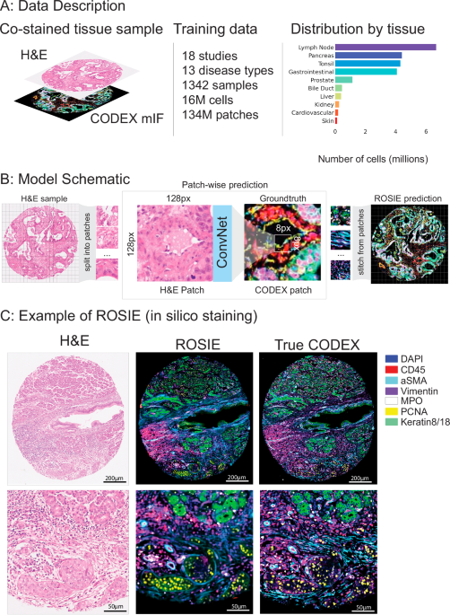
我们在20项研究中介绍了一个培训和评估数据集（图。 1a，桌子 1;有关数据集详细信息，请参见补充材料）。训练数据集由18个研究，1342个样本和13种疾病类型的16多个细胞组成。评估数据集由4个研究，485种样本和4种疾病类型的5个细胞组成。两项研究（Stanford-PGC和Uchicago-DLBCL）在培训和评估数据集之间进行了分配。所有研究均对完全相同的样品进行H＆E和法典的组织样品进行了染色。除Uchicago-dlbcl外，所有数据集均由组织微阵列（TMA）核（平均10 K细胞）组成，其中包含完整的幻灯片样品（平均每片平均1.5 m细胞）。Stanford-PGC是一项针对斯坦福医疗保健的胰腺和胃肠道癌患者的研究。Ochsner-CRC是Ochsner医疗中心的结直肠癌患者的研究。Tuebingen-Gej是一项研究，该研究是Tã¼bingen大学医院胃食管交界处的癌症患者。Uchicago-DLBCL是对芝加哥大学医学中心弥漫性大B细胞淋巴瘤患者的研究。

一个我们的培训数据集由18个研究和16个M细胞组成。每个组织样品均与H＆E和Codex共染色。该数据集中有16种疾病类型和10种身体区域。右侧显示了跨培训和评估数据集的代表组织类型的总体分布。b显示了模型训练和推理的示意图。给定H＆E样本，图像被分为尺寸128px x 128px的斑块。对模型进行了训练，以预测相应的法典图像中中心8px x 8px补丁的平均表达式。训练模型后，通过将所有生成的补丁汇总到单个图像中来生成预测的法典图像。c鉴于H＆E染色的图像，Rosie预测了50个生物标志物的像素级表达。可视化了一个模范图像（具有最高的皮尔森R得分），其中有七个代表性的生物标志物，并与真实的法典图像一起显示。虽然我们分析中使用的生成图像是通过8PX步骤产生的，但该图像是使用1PX步骤制作的，以更高的视觉清晰度。

从H＆E染色推断蛋白质表达的生成深度学习模型

罗西（Rosie）是基于H＆E图像在样品上进行硅染色的框架。使用Convnext²⁷卷积神经网络（CNN）体系结构，Rosie在斑块级别运行：给定输入128 - 128像素贴片，它可以预测整个中心8â€8像素的生物标志物面板的平均表达式（图图） 1B）。使用具有8px步长的滑动窗口，我们迭代在样品中的所有8 8像素贴片上进行预测，然后缝制预测以产生整体，连续的图像。Rosie可以使用较小的滑动窗口尺寸运行，以降至1PX，以获取本机分辨率输出（请参阅补充图。 5例如）。由于计算权衡，本文进行的分析在标准的8PX滑动窗口设置上。虽然视觉变压器（VIT）模型²⁸最近，作为表现最佳的组织病理学基础模型，我们发现，尽管尺寸较小，但我们发现Convnext优于几个VIT模型（补充表 1）。

在所有研究中，共有148种独特的生物标志物。我们限制了通过患病率预测前50个生物标志物的方法。尽管这50个生物标志物对所有评估研究都染色，但培训中使用的一些研究却没有。在这些情况下，仅使用此组中存在的生物标志物的子集。完整的生物标志物设置了该模型的预测包括（按照率的顺序）：

DAPI, CD45, CD68, CD14, PD1, FoxP3, CD8, HLA-DR, PanCK, CD3e, CD4, aSMA, CD31, Vimentin, CD45RO, Ki67, CD20, CD11c, Podoplanin, PDL1, GranzymeB, CD38, CD141, CD21, CD163, BCL2, LAG3,EPCAM，CD44，ICOS，GATA3，GAL3，CD39，CD34，TIGIT，ECAD，CD40，VISTA，VISTA，HLA-A，MPO，MPO，PCNA，PCNA，ATM，TP63，IFNG，KERATIN8/18，IDO1，IDO1，CD79A，CD79A，HLA-E，HLA-E，COLLAGENIV，COLLAGENIV，CD666666666666666666。

Rosie准确预测蛋白质生物标志物表达式

在将Rosie应用于四个评估数据集时，我们报告了Pearson R相关性为0.285，Spearman R相关性为0.352，在比较所有四个数据集中所有50个生物标记物（表）时（表比较地面真相和计算产生的表达式时）的样本级别的C折射率为0.706（表）（表 2）。Pearson相关性表示线性预测关系，而Spearman R和C指数表示预测表达在临床任务中的有用性，涉及通过表达某个生物标志物来订购细胞或样品的临床任务（例如，在癌症患者中识别免疫标记物）。C-指数是指使用第75个百分位表达值作为阈值在样本级别计算的一致性指数。例如，C-指数为0.5表示随机机会。我们表明，我们的方法明显优于两种基线方法：H＆E表达它使用RGB通道的平均强度作为每个生物标志物蛋白质表达的直接代理，旨在测试我们的预测精度是否仅仅是由于概括了染色信号。和细胞形态它使用从细胞分割的形态特征除了三个RGB通道作为多层感知器（MLP）神经网络的输入，该网络训练了预测蛋白质表达，它旨在用作代表性的机器学习模型，该模型使用常见的H＆e-e-e-e-e-e-e-e-e-e-e-e-e-e-e-e-e-e-e-e-eDer的特征作为输入。两种基线方法都基于三个评估指标均报告了近乎交战的性能。图 1C可视化示例预测的样品具有代表性的七个生物标记面板。最后，我们使用Pix2Pix训练和评估生成对抗网络（GAN）²⁹模型架构预测法典表达并表明这种方法的表现显着不足Rosie（补充表 1，补充图 11）。

罗西（Rosie）生成了高度准确的全样本法典图像，并概括了代表性免疫和结构生物标志物面板的显着视觉特征（图 2a）。为了说明Rosie在一系列预测中的鲁棒性，包括相对较低的预测，我们在斯坦福-PGC数据集中显示了从第99、75、75、50、50和25％的性能（Pearson R）中绘制的并排预测和地面真相样本。图 2b显示了所有评估数据集中的50个预测的生物标志物中的每个预测生物标志物中的每一个。我们还单独地可视化每个生物标志物（补充图。 1）来自Stanford-PGC（Pearson R的中位样品），以及Pearson R的分布（补充图。 2）和等级测试的分数（Spearman R和C-Index，补充图。 3）。

一个预测和测量的法典样本以及共同染色的H＆E图像。显示了第99，第75，第50和25个百分位（由Pearson R）样本显示，颜色为七个结构（keratin8/18，Epcam，epcam，epcam，ecad，ecad，asma，cd31，panck）和Immune（hla-e，hla-e，hla-e，gal3，gal3，gal3，gal3，cd45，cd45，cd45，cd45，cd21，lag3，cd66，cd66，cd66，cd68）。b所有评估数据集的Pearson R相关性（可视化的生物标志物已彩色）。补充图 5可视化预测的缩放补丁。c来自其他三个数据集的中位样品的可视化（Pearson R）：Ochsner-CRC，Tuebingen-Gej和Uchicago-DLBCL。为了解释Rosie产生的预测，我们应用了Grad-CAM

30^{，一种针对CNN的视觉解释性技术，从斯坦福-PGC数据集的随机采样H＆E图像贴片上，以查看图像中的模型在做出预测时引起注意的位置。}补充图 10可视化从随机采样图像贴片中为10个生物标志物生成的梯度热图。我们观察到，对于主要由核蛋白表达（例如DAPI，KI67，PCNA）确定的生物标志物，热图值位于斑块的中心周围。相反，对于可能更依赖上下文依赖性的生物标志物（例如CD68，Panck，ECAD），热图值更加分散，并且位于细胞邻域周围。

对看不见的研究和疾病类型的概括

Rosie在训练期间从未见过的临床部位和疾病类型的样品进行评估，即使对疾病的样本进行了良好的表现。When evaluated on Ochsner-CRC and Tubingen-GEJ, two studies whose samples and disease types do not appear in the training dataset, ROSIE reports comparable average performance to Stanford-PGC: a Pearson R of 0.241 (vs. 0.319 on Stanford-PGC), Spearman R of 0.283 (vs. 0.386 on Stanford-PGC), and a sample-level C-index of 0.633（在斯坦福 - pgc上的0.694 vs. 0.694）遍布所有50个生物标志物（请参阅Tableâ 2）。我们在图中视觉上确认了这些结果。 2C，其中包含来自其他三个评估数据集（Ochsner-CRC，Tuebingen-Gej和Uchicago-dlbcl）的中位样品（由Pearson R）。

我们还验证了使用Orion成像的大肠癌数据集上的Rosie的性能，该数据集是多重的免疫荧光平台³¹。该数据集（Orion-Crcâ）由共同染色的，配对的H＆E和MIF全幻灯片图像（WSIS）组成。在我们的分析中，我们从5个WSIS中对50台乘以3000px样品进行了对Rosie的预测性能，以使用Spearman等级相关性测量Rosie的17个重叠蛋白生物标志物的预测性能。补充图 8表明，在由与法典不同的MIF成像平台产生的数据集上，Rosie在生物标志物的一个子集中表现良好，但在几种生物标志物（例如ECAD）中也挣扎。

一个简单的度量标准，用于在硅染色质量中进行后处理和过滤

由于染色质量，组织类型和人工制品等因素，批处理效应或组织病理学样本之间的变化可能会显着影响深度学习模型的推广性。^{32，，，，33}。因此，可以预测由于批处理效应而将哪些样品质量较低，并将其排除在下游分析之外是可取的。

为此，我们介绍了两个简单但有效的启发式方法，以在染色质量上进行预测的样本：动态范围，这是对生物标志物染色中第99个百分位数值之间差异的量度；和W1距离，这是测试H＆E图像直方图分布与所有直方图分布之间的平均瓦斯汀距离。补充图 6显示了将每个质量过滤器应用于四个评估数据集的效果：使用W1距离使用中位数作为截止分布样品的截止，Pearson R得分从0.285增加到0.312，使用动态范围为0.336。补充图的面板A 6说明了动态范围与皮尔森R得分之间的关系。面板B同样显示了预测的瓦斯坦距离与皮尔森R得分之间的关系。

生物标志物预测可用于细胞和组织表型

鉴于Rosie产生的蛋白质生物标志物表达与地面真相测量高度相关，因此我们通过在表型细胞中使用它们来验证它们的生物学和临床实用性。为此，我们首先训练最近的邻居算法，以预测地面真相法典生物标志物表达式上带有的细胞标签。然后，我们将Rosie生成的生物标志物表达式输入到算法中以产生细胞类型的预测。Rosie可以比使用细胞形态和H＆E RGB通道（作为输入的模型）预测七种细胞类型（B细胞，内皮细胞，上皮细胞，成纤维细胞，巨噬细胞，中性粒细胞和T细胞）明显好得多（细胞形态）或根据平均样品比例随机分配细胞类型（散装表型）（图 3）。进一步的分析表明，B和T细胞分化与细胞类型分类混淆矩阵的分化（补充图。 4）。此外，我们在Ochsner-CRC数据集上执行细胞表型，发现Rosie产生的标签 -与斯坦福-PGC相当的生物标志物（平均F1分别为0.411和0.507）（补充表分别为0.411和0.507） 2和补充图 4）。图3：使用Rosie进行细胞类型预测。

F1分数（n在主要的Stanford-PGC数据集上，将Rosie与两个基线的性能进行比较：817,765个细胞）。散装表型，它根据样品级单元格的比例随机分配细胞类型，并且形态特征，它使用三层神经网络根据形态特征和H＆E RGB通道对细胞进行分类。数据表示为带有误差线的平均值，作为95％的自举置信区间。bPearson R.从十二个中位样品中的细胞表型预测的可视化。我们还评估了表现最好的细胞表型算法，Cellvit+++

34^{，并将其与罗西的表现进行比较。}Cellvitâ++是一种视觉变压器模型，该模型在H＆E图像上训练以预测细胞表型。要进行并排评估，我们使用已在蜥蜴数据集上训练的模型检查点³⁵并将细胞类型从蜥蜴和Rosie调和六类：B细胞，结缔组织，上皮，中性粒细胞，T细胞等。补充图 9表明罗西（Rosie）在从斯坦福-PGC数据集中预测这些细胞类型方面优于Cellvit++。

我们对这些预测是否验证组织之间的治疗相关区别感兴趣。通常已知不同的组织类型在免疫学上是热的，表明免疫细胞的存在和浸润更大，或者较冷，这意味着免疫细胞活性较小。例如，已知胰腺癌（例如Stanford-PGC数据集）较冷，而结直肠癌（例如Ochsner-CRC数据集）已知很炎热。^{36，，，，37}。实际上，我们的结果反映了这种免疫有效性检查，在免疫学上，较冷的斯坦福-PGC的预测平均每样本的平均比例为20.0％（vs. 21.1％地面真相），而在免疫学上，Hotter-ochsner-ochsner-ochsner-ochsner-crc具有每个样品40.1％T细胞（vs. 30.6％地面真相）。

我们还将方法扩展到了单细胞表型，并证明了其在识别样品中组织结构方面的有效性。我们使用表现最佳的组织结构识别算法，SCGP³⁸，将获得的组织样品投射到图中，并以细胞和边缘为相邻细胞对的节点。使用此图结构，该算法会根据地面真理和Rosie生成的生物标志物表达式进行无监督的聚类来发现组织结构。图 4通过比较地面真相和产生的表达式，显示了几个样品中发现的结构以及报告的调整后的兰德指数（ARI）和F1得分。我们的方法分别达到平均ARI和F1评分为0.475和0.624，并且使用细胞形态分割和平均H＆E ERGB值衍生而成的细胞形态特征，高于从三层神经网络产生的表达式的基线方法（ARI为0.105和F1，为0.105和F1）。在补充表中报告了全部分数 3。

使用Rosie在Stanford-PGC测试数据集中生成的生物标志物发现组织结构。使用图形分配算法鉴定了五个组织结构，该算法根据细胞的表达谱和相邻细胞来簇。该算法是在测量的地面真相和Rosie上执行的 -生成的生物标志物表达式，然后与共同的标签集进行调和。一个可视化使用地面真相法典测量结果Rosie发现的几种代表性的组织结构样本 - 生成表达式和形态基线方法。b左：我们报告F1分数（n= 635,649个细胞）通过比较使用地面真相，Rosie生成的生物标志物和形态特征发现的结构。数据表示为带有误差线的平均值，作为95％的自举置信区间。右：还通过比较未标记的发现群集来报告ARI分数，其中每个点都是样本。盒子图显示了中值（中心线），第25个和第75个百分位数（框边缘）以及最小值和最大值。

另外，我们使用Rosie -产生的表达式以识别两个感兴趣的细胞邻域表型：肿瘤浸润淋巴细胞（TILS）和淋巴细胞相邻上皮细胞（LNE）。这些细胞类型由它们的细胞生态位及其生物标志物表达谱定义：tils是驻皮组织中的淋巴细胞，而LNES是邻近淋巴细胞的上皮细胞。图 5shows that the predicted proportions of TILs and LNEs per sample in the Stanford-GPC test dataset are highly correlated with the ground truth-derived proportions (Pearson R of 0.805 and 0.598 and Spearman R of 0.329 and 0.575 for TILs and LNEs, respectively), suggesting that the ROSIE-generated expressions may be useful for clinical tasks that involve estimating or ordering samples in a patient通过特定生物标志物，细胞或细胞相互作用的存在。

我们确定了感兴趣的两个细胞邻域表型：肿瘤浸润淋巴细胞（TIL）和淋巴细胞相邻上皮细胞（LNE）。TIL被定义为被标记为淋巴细胞（B和T细胞）并驻留在上皮组织（使用图分配算法）的细胞。LNE是至少有一个淋巴细胞作为邻居的上皮细胞。将TIL测量为每个样品的原始计数，而LNEs则测量为淋巴细胞邻居的上皮细胞比例。一个我们根据地面真理和罗西预言的表达方式可视化tils和lnes的三个样本（由皮尔森中间）。b预测和地面真实测量值的散点图，每个点代表样本。

我们的研究旨在弥合丰富，廉价的H＆E染色与多重免疫荧光（MIF）染色提供的丰富但昂贵的分子信息之间的差距。我们提出的主要问题是H＆E染色在多大程度上嵌入了可以在计算上提取的分子标志和特征。我们的结果表明，尽管H＆E染色在识别很少的细胞表型方面受到限制，但是当用深度学习生成的AI方法分析时，其结构和形态学特征确实包含有关蛋白质表达的重要信息。这表明H＆E染色具有未实现的潜力，可以在传统上需要更复杂和昂贵的测定法中使用。尽管先前的工作一次重点是一次归档多个标记，但我们的研究是第一个使用深度学习来学习H＆E和多达50种蛋白质生物标志物之间的关系。现在，此设置可以对组织微环境有更全面的视野，并对特定肿瘤和免疫细胞表型提供了更多细微的见解。

基于变压器体系结构的基础模型的最新进展接受了组织病理学图像的培训^{10，，，，12，，，，39}适应和微调在各种临床下游任务上进行调整和微调时表现出希望。但是，我们的结果表明，这种模型的表现仍然不足我们明显较小的卷积神经网络。例如，在组织病理学图像上预先训练的300次参数的VIT-L/16变压器模型仍然不如Convnext（50 m参数CNN）在非病理学图像上进行了训练。实际上，大规模研究比较基础和特定于任务的模型⁴⁰发现较小的特定于任务的模型通常比基础模型的模型经常优于基础模型，尤其是在具有足够标记的培训数据的情况下。此外，由于其较大的模型尺寸，基于变压器的基础模型在训练上的计算量明显更高。我们为这一违反直觉发现提供了几种潜在的解释：首先，CNN中卷积操作的感应偏见更适合从基于斑块的组织学成像中提取局部上下文特征；其次，较大的基础模型更难训练，并且可能对训练数据更容易过分，我们观察到，与CNN相比，该过程中更大的视觉变压器模型的性能要早。该结果表明，未来研究在分析大型基础模型何时比较小的CNN更合适的情况下的重要性。

我们进一步证明，我们的像素级基于CNN的方法在准确性和训练稳定性方面都优于基于GAN的方法。虽然甘恩在硅染色中已被用于，但它们面临几个局限性：（1）先前文献的评估主要集中在视觉指标上，主要是SSIM，而不是生物学上有意义的准确性，（2）由于最小值优化过程，训练过程中的不稳定性，尤其是当共同预测生物标志物的大型小组时（补充生物标记图。 11），以及（3）基于贴片的H＆E输入处理引入的边界伪影。相比之下，我们的模型训练具有单个稳定的MSE损失，并有效地缩放到50 plex生物标记面板。

我们研究的一个重点是我们生成的表达和细胞表型的等级相关性。Strong rank correlations suggest that the generated biomarkers are useful in clinical settings where the relative ordering of the presence of a biomarker or phenotype is important, e.g., finding patients that are the most receptive to a therapy or predicting patient prognosis based on a specific biomarker.For instance, we observe that while our model can effectively predict cell neighborhood phenotypes (TILs and lymphocyte neighboring epithelial cells), these predictions also exhibit biases in over- or under-predicting the proportion or counts of these phenotypes.Despite these biases, the relative ordering of these phenotypes is still largely maintained and thus is still useful in the settings mentioned above.

Inter-batch effects due to staining technique, quality, and machinery are known to cause variations in the image statistics of H&E stains.Since predictions generated on H&E stains that significantly deviate from the training data are expected to perform worse, we propose two methods for quantifying the quality of generated mIF stains.We demonstrate that computing the dynamic range of predicted expressions and calculating the Wasserstein distance between training and generated data image histograms both correlate well with the empirical prediction accuracy.We believe these can be valuable tools that accompany our deep learning framework, allowing users to determine their clinically acceptable range of stain generation quality.

We acknowledge several limitations with our data and framework.Though we perform quality control on each sample (see Supplementary Methods), the alignment of H&E and CODEX images is susceptible to artifacts such as fraying, which can lead to misalignments and affect the accuracy of predictions.Second, not every biomarker is equally represented in the training data—this data imbalance is one reason why our performance on certain biomarkers is poor.We attempted to mitigate this by oversampling underrepresented biomarkers but did not observe significant improvement over equal sampling.As a result, we focus our phenotyping analysis on using the top 24 biomarkers, where performance is the most robust.Nonetheless, we observed experimental benefit from training on the full 50-plex panel versus a smaller panel (e.g., 10 and 24) even when evaluating only on the smaller panels.We hypothesize that training on a larger set encourages information sharing between the neural network layers and thus improves the overall predictive performance on the analyzed subset.An additional benefit of this approach is that in the ConvNeXt model architecture, all biomarkers are predicted from a shared embedding space (penultimate layer of the model), so biomarkers that are related to or a subset of other ones share the same representations in the model.

Another potential limitation in our approach is that there are limited context windows around cells.Given the model constraints, we experimented with larger context windows (i.e. 256 × 256px) but did not improve model performance.At the standard 40x magnification for H&E scanning, our current 128 × 128px window typically includes around thirty cells or a 3-hop neighborhood of cells, which would include information about not only the center cell but its surrounding niche.Additionally, all data collected and imaged in our study was performed in-house on the same experimental setup (e.g., H&E scanner, PhenoCycler Fusion).Due to this uniformity, we have limited experimental evidence demonstrating our model’s robustness on data sourced from significantly different environments, as batch effects from different reagents and protocols would be expected to be more significant.Our evaluation on the Orion-CRC dataset highlights the performance of ROSIE when pushed to the boundaries of generalizability (different imaging platform, disease type, and clinical site): while we observe robust prediction on some biomarkers (e.g., CD45), other biomarkers underperform (e.g., ECad).These results imply fundamental limitations of ROSIE to easily generalize across multiple sources of variability without additional adaptation such as re-training.We look forward to additional validation of our method as more paired H&E/mIF data is made publicly available.

Due to the variability in biomarker performance across the full panel, ROSIE is not an appropriate replacement for a full-panel CODEX experiment.The primary aim of our method of training on the full 50-biomarker panel is to 1. maximize the amount of signal available to the model via information sharing from different markers, and 2. determine in an unsupervised manner which markers are the most predictive.The inherent limitations of H&E staining mean that resolving certain protein expressions (e.g., immune markers) are difficult without additional assaying.However, we demonstrate that ROSIE can still reveal significantly more information compared to the H&E stain alone.

Our study demonstrates a method for extracting multi-plex spatially resolved protein expression from H&E stains.Given the ubiquity of H&E staining in clinical workflows, a framework for enabling in silico staining of dozens of spatially resolved protein biomarkers offers enormous potential for improving clinical workflows and decision-making.In silico staining can reduce the need for costly immunostaining assays, significantly decreasing turnaround time and associated clinical costs.Additionally, it can serve as a screening tool using existing H&E slides from patient cohorts, enabling clinicians to prioritize patients based on predicted therapeutic responses.Finally, in resource-limited settings, in silico staining can democratize access to advanced biomarker assays that would otherwise be unavailable.We hope that future validation and continued improvements to ROSIE will enable these use cases to be realized in real-world clinical settings.

Patient samples and data were obtained using institutional protocols.

CODEX data collection

All samples are prepared, stained, and acquired following CODEX User Manual Revc。Coverslip preparation

Coverslips are coated with 0.1% poly-L-lysine solution to enhance adherence of tissue sections prior to mounting.

The prepared coverslips are washed and stored according to the guidelines in the CODEX User Manual.

Tissue sectioning

formaldehyde-fixed paraffin-embedded (FFPE) samples are sectioned at a thickness of 3-5 μm on the poly-L-lysine coated glass coverslips.

Antibody conjugation

Custom conjugated antibodies are prepared using the CODEX Conjugation Kit, which includes the following steps: (1) the antibody is partially reduced to expose thiol ends of the antibody heavy chains;(2) the reduced antibody is conjugated with a CODEX barcode;(3) the conjugated antibody is purified;(4) Antibody Storage Solution is added for antibody stabilization for long term storage.Post-conjugated antibodies are validated by SDS-polyacrylamide gel electrophoresis (SDS-PAGE) and quality control (QC) tissue testing, where immunofluorescence images are stained and acquired following standard CODEX protocols, then evaluated by immunologists.

Staining

CODEX multiplexed immunofluorescence imaging was performed on FFPE patient biopsies using the Akoya Biosciences PhenoCycler platform (also known as CODEX).5 μm thick sections were mounted onto poly-L-lysine-treated glass coverslips as tumor microarrays.Samples were pre-treated by heating on a 55 °C hot plate for 25 minutes and cooled for 5 minutes.Each coverslip was hydrated using an ethanol series: two washes in HistoChoice Clearing Agent, two in 100% ethanol, one wash each in 90%, 70%, 50%, and 30% ethanol solutions, and two washes in deionized water (ddH2O).Next, antigen retrieval was performed by immersing coverslips in Tris-EDTA pH 9.0 and incubating them in a pressure cooker for 20 minutes on the High setting, followed by 7 minutes to cool.Coverslips were washed twice for two minutes each in ddH2O, then washed in Hydration Buffer (Akoya Biosciences) twice for two minutes each.Next, coverslips were equilibrated in Staining Buffer (Akoya Biosciences) for 30 minutes.The conjugated antibody cocktail solution in Staining Buffer was added to coverslips in a humidity chamber and incubated for 3 hours at room temperature or 16 hours at 4 °C.After incubation, the sample coverslips were washed and fixed following the CODEX User Manual.Additional antibody information including clone name, barcode number, and reporter name is available at:https://gitlab.com/enable-medicine-public/rosie/-/blob/main/Antibody%20Information.xlsx。Data acquisition

Sample coverslips are mounted on a microscope stage.

Images are acquired using a Keyence microscope that is configured to the PhenoCycler Instrument at a 20X objective.All of the sample collections were approved by institutional review boards.

To correct for possible autofluorescence, “blank” images were acquired in each microscope channel during the first cycle of CODEX and during the last.For these images, no fluorophores were added to the tissue.These images were used for background subtraction.Typically, autofluorescence will decrease over the course of a CODEX experiment (due to repeated exposures).Thus, to correct each cycle, our method determines the extent of subtraction needed by interpolating between the first and last “blank” images.

Sample preprocessing

Samples are first stained and imaged using CODEX antibodies on the Akoya Biosciences PhenoCycler platform and then stained and imaged with H&E on a MoticEasyScan Pro 6 N scanner with default settings and magnification (40x).The CODEX DAPI channel and a grayscale version of the H&E image are used to perform image registration.Both images have their contrast enhanced using contrast-limited adaptive histogram equalization.The SIFT features⁴¹of each image are then found and matched based on the RANSAC algorithm⁴²to find an image transformation from the H&E image to the CODEX coordinate space.The transformation was limited to a partial affine transformation (combinations of translation, rotation, and uniform scaling).If the initial alignment based on the grayscale H&E image was not successful, the process was repeated using the nuclear channel of the deconvolved H&E image (using a predetermined optical density matrix⁴³) or individual color channels of the H&E image.The H&E stains were performed centrally on-site using standard staining protocols.However, inter-user variability such as staining durations and slide handling techniques may have contributed to batch effects.Such variability introduces potential sources of technical heterogeneity, which could impact the consistency of tissue staining quality and consequently influence downstream analytical results.

Training details

The training process is visualized in Fig. 1B。Each sample was first split into patches.In our standard approach, we subdivided a sample into non-overlapping 8x8px patches.The average expression within each patch is computed for every CODEX biomarker.Then, a 128 by 128px H&E patch is extracted centered on the 8x8px patch, which is used as input to the model.Thus, for instance, a 1024px by 1024px sample would yield a prediction of 128px by 128px resolution, as each 8px by 8px patch is represented by a single pixel prediction.Our model is based on a ConvNext-Small architecture with 50 M parameters.The model is pre-trained on the ImageNet image dataset.During training, random augmentations are performed: horizontal and vertical flipping, brightness, contrast, saturation, hue jittering, and normalization are all performed.The training task consists of the model predicting the mean expression of the center 8 × 8px of a 128 × 128px patch for each biomarker.Thus, the model performs multitask regression (i.e., a 50-length vector) for a given patch.Model validation during training is performed using two metrics: Pearson R and SSIM (Structural Similarity Index Measure).Pearson R is a correlation metric used to assess the similarity between the measured and predicted expressions;SSIM is a similarity metric that assesses the qualitative similarity between two samples.Pearson R is computed across patches, while SSIM is computed on the reconstructed samples.This is to evaluate the model’s predictions both in terms of biological accuracy and visual similarity.

Each study has a different biomarker panel, so to account for missing biomarkers, we used a masked mean squared error loss where only the loss over present biomarkers is computed.

Training is performed on 4 V100 GPUs with a batch size of 256 and a learning rate of 1e-4 with the Adam⁴⁴optimizer on a schedule that reduces by half every 30 K iterations.Models are trained until no improvement in this metric is observed for 75 K steps.On the same hardware, evaluation of a single TMA core takes approximately 5 minutes.Given that the ConvNext model is relatively lightweight ( ~ 50 M parameters), it can also be deployed on a single on-premise, consumer-grade GPU or CPU.Model training and evaluation are performed with Python using the torch⁴⁵, pytorch-geometric⁴⁶, scikit-learn⁴⁷, and scipy⁴⁸packages.

A description of the different studies comprising the full training dataset, including disease type, number of cells and samples, and biomarker panel, are available athttps://gitlab.com/enable-medicine-public/rosie/-/blob/main/Training%20Datasets.csv。Sample generation

Inference is performed on the foreground H&E patches and then stitched into the predicted sample.

In the standard analyses presented, a stride of 8px is used, which produces a predicted image that is 8x downsampled from the original image size.This produces predictions at a resolution of 3.02 microns per pixel.Using this image, we then produce cell-level expression predictions by upsampling the predicted image to the native resolution and then computing the average expression per cell based on the cell segmentation mask.The ROSIE-generated images are saved in TIFF image format, which are identical to the CODEX-measured images.Thus, any downstream analyses that can be performed on CDOEX data can similarly be performed on ROSIE-generated data.

To produce higher-resolution images, we also demonstrate the predictions using 1px strides.In this setting, overlapping patches are generated at 64x the number of total predictions.This setting produces predictions at a resolution of 0.3775 microns per pixel.The resulting images are demonstrated and compared to the standard 8px setting in Supplementary Fig. 5。质量控制We introduce two quantitative metrics for determining whether an H&E sample is in distribution and a high-quality generation.

First, we measure the deviation between the image intensity distributions of a test H&E sample and the H&E samples in the training data.

For a given test and training image pair, we extract 256 histogram bins from the image to obtain discrete distributions and then compute the Wasserstein (or Earth Mover’s) distance (also called W1 distance) between the two distributions.The quality metric for a given test image, then, is computed as the average W1 distance across all training images.By using this metric, we can a priori determine whether a test sample is in distribution and appropriate for evaluation.

Additionally, at the biomarker channel level, we use the dynamic range as a simple proxy for estimating the quality of a predicted sample.Since channels with very low maximum expression correlate with poor quality acquisitions (due to artifacts, staining issues, etc.), we set a threshold below which we exclude biomarkers from evaluation.Dynamic range is computed as the difference between the 99th and 1st percentile values in a generated biomarker stain.Since the dynamic range is only a function of the predicted image, it does not depend on having ground truth CODEX measurements for an H&E sample.

Expression metrics

We report three primary evaluation metrics for patch-level predictions: Pearson R (sklearn.metrics.pearsonr), Spearman R (sklearn.metrics.spearmanr), and concordance index, or C-index (lifelines.utils.concordance_index).Pearson correlation is a measure of the linear relationship between the ground truth and predicted biomarker expressions.Additionally, we report two rank metrics (Spearman R and C-index) to assess the model predictions’ usefulness in clinical tasks that rely on ordering patient samples by a specific biomarker expression or cell type count.Pearson and Spearman correlations are calculated as the average correlations across all ground truth and predicted CODEX patches.C-index is computed on the 75th percentile values for both ground truth and predicted CODEX for each biomarker and across all samples.Only during training, SSIM is computed across ground truth and predicted images.To ensure that the metrics are calculated on valid data points, we exclude patches with a lower groundtruth expression value than the 90th percentile value of background noise for each biomarker.

基线方法

We also introduce several baseline methods for comparison to ROSIE:

First, we use the H&E sample alone to predict CODEX expression (calledH&E expression)。In this method, we apply a simple threshold ( > 50), averaged across the three color channels, and then use the intensity to predict each biomarker.This is to evaluate the similarity of the hematoxylin and eosin stains to the CODEX stains and to validate that the model is not simply recapitulating stain intensity in its CODEX predictions.

Second, we compute morphology statistics based on the segmentation masks calculated from the DAPI channel (calledcell morphology)。Cell segmentation is performed using the DeepCell algorithm⁴⁹。We use the HistomicsTK compute_morphometry_features function and extract 19 features in total: Orientation, Area, Convex Hull Area, Major Axis Length, Minor Axis Length, Perimeter, Circularity, Eccentricity, Equivalent Diameter, Extent, Minor to Major Axis Ratio, Solidity, Hu Moments (1st to 7th).In addition, we compute the average across each of the RGB channels and include these as three additional features.We train a three-layer multi-layer perceptron neural network using these features as input to predict the expression of 50 protein biomarkers.Each layer has 100 nodes followed by a ReLU activation function and is trained with a 1e-4 learning rate, mean squared error loss, and Adam optimizer.The weights that generated the best validation accuracy after 50 epochs are used.This is a stronger baseline that is intended to represent typical features (morphology and intensity) derived from H&E images.Finally, as an additional baseline for cell phenotyping, we assign cell labels randomly according to the average ground truth cell label proportions across all samples (calledbulk phenotyping)。This method approximates estimating cell type proportions through a cheaper, more readily available phenotyping technique than CODEX (like flow cytometry) and then using them to infer spatially located cell types.

To train the pix2pix GAN model, we use the pix2pix model architecture²⁹and software package and randomly sample 256px by 256px H&E and CODEX patches from the Stanford-PGC training dataset.The model is trained to predict the 50-channel CODEX output image based on the H&E input.The model is trained for 50 epochs with 100 patches randomly chosen from each sample.The full implementation and code are provided in the Gitlab repository.

Cell phenotyping

Cell phenotyping metrics are computed using the following steps: First, cell clusters are produced using Leiden clustering based on the cell-level CODEX measured expressions.These clusters are identified and merged based on cell expression within each cluster to produce manually annotated cell labels.Then, we trained a k-nearest neighbors algorithm (where k = 100) to generate a graph based on these clusters, which is used to automatically generate the reference cell labels.To prevent class imbalance, we sample from each cell label class with equal proportion for the training set.We use the same kNN and the predicted expressions to generate the predicted cell labels.We report the F1 scores, which are relative to the cell typing determined using clustering on the法典measurements.In this analysis, we use only the top 24 biomarkers by Pearson correlation as input features to the kNN algorithm.Supplementary Fig. 7shows the mean biomarker expressions for each defined cell type.For cell phenotyping performed on Ochsner-CRC, we similarly train a kNN on manually annotated cell labels and use it to generate reference cell labels.For uniformity of comparison, we define the same cell phenotypes as in the Stanford-PGC dataset.

To perform a cell phenotyping comparison with CellViT + +, we use the model checkpoint that has been trained on the Lizard dataset³⁵since the cell definitions most closely match the set derived in our analyses.We reconcile the cell types from Lizard and ROSIE into six categories: B cells, connective, epithelial, neutrophils, T cells, and other.Given that the CellViT + + algorithm jointly performs segmentation and phenotyping, we also reconcile the cell segmentations produced by the algorithm and our DAPI-derived segmentations by only including the intersecting set of cells from both sets.This yields a total of 220 K cells when evaluated on the Stanford-PGC evaluation dataset.

Tissue structure discovery

The Spatial Cellular Graph Partitioning (SCGP) framework³⁸is summarized in the following steps:

1. 1。

   Construct a graph with cells as nodes.Spatial edges are added between neighboring cell pairs, and feature edges are added for cell pairs with similar expression profiles.

2. 2。

   Partitions are detected by community detection algorithms such as the Leiden algorithm⁵⁰。

3. 3。

   Each partition is manually annotated based on its underlying expression profile and cell morphology.

The above steps are performed independently on the ground truth and H&E imputed mIF samples, and a mapping from the imputed partitions to the ground truth partitions is calculated.Finally, we compute the adjusted Rand Index (ARI) and F1 scores.ARI measures the similarity between the ground truth and imputation-derived partitions and does not require cluster labeling;the F1 score is computed over manually annotated labels.As a baseline, we perform the partitioning over morphology features extracted from the cell segmentations, as well as adding in the average RGB expressions per cell.Supplementary Fig. 7shows the mean biomarker expressions for each defined tissue structure.

Cell neighborhood phenotyping

To define cell neighbors, we first perform cell segmentation on the DAPI channel for each sample.Based on the computed cell centroids, we then construct a Delauney triangulation and Voronoi diagram, from which we then construct a graph with cells as nodes and Delauney neighbors as edges.To define lymphocyte neighboring epithelial cells, we identify epithelial cells and then find the subset of these cells that share an edge with a lymphocyte (B cell or T cell).The reported percentage of LNEs is defined as the proportion of epithelial cells in a sample that are LNEs.Additionally, we define tumor-infiltrating lymphocytes (TILs) as lymphocytes embedded in tumor regions.To identify TILs, we find lymphocytes that are assigned to epithelial tissue structures.For each sample, we report the raw count of TILs.

Gradient heatmaps

To interpret how ROSIE generates biomarker predictions from H&E images, we apply Gradient-weighted Class Activation Mapping (Grad-CAM)³⁰to visualize the spatial regions within an input patch that influence the model’s predictions.Specifically, we use the gradients of each biomarker’s output with respect to the final convolutional feature maps to compute a weighted sum of activations, producing a heatmap that localizes the regions most relevant to the prediction.These gradients are globally average-pooled across the spatial dimensions to obtain a set of weights, which are then multiplied by the corresponding activation maps, summed, and upsampled to produce a localization map.

Statistics and reproducibility

No statistical method was used to predetermine sample size.No data were excluded from the analysis after initial aggregation of the full training and evaluation datasets.Data splits (e.g., training, validation, testing) were performed on the coverslip level, with splits randomly chosen among coverslips.The investigators were not blinded to allocation during experiments and outcome assessment.

报告摘要

Further information on research design is available in the Nature Portfolio Reporting Summarylinked to this article.

The full code repository, including files for evaluating ROSIE, are available athttps://gitlab.com/enable-medicine-public/rosie。参考

Authors and Affiliations

1. Enable Medicine, Menlo Park, CA, USA

   Eric Wu, Matthew Bieniosek, Zhenqin Wu, Alexandro E. Trevino, Aaron T. Mayer & James Zou

2. Department of Electrical Engineering, Stanford University, Stanford, CA, USA

   Eric Wu & James Zou

3. Department of Computer Science, Stanford University, Stanford, CA, USA

   Nitya Thakkar

4. Department of Pathology, Stanford University, Stanford, CA, USA

   Gregory W. Charville

5. Department of Pathology and Neuropathology, University Hospital and Comprehensive Cancer Center Tübingen, Tübingen, Germany

   Ahmad Makky & Christian M. Schürch

6. Cluster of Excellence iFIT (EXC 2180) “Image-Guided and Functionally Instructed Tumor Therapies”, University of Tübingen, Tübingen, Germany

   Christian M. Schürch

7. Public Health Sciences Division, Fred Hutchinson Cancer Center, Seattle, WA, USA

   Jeroen R. Huyghe, Ulrike Peters & Christopher I. Li

8. Department of Epidemiology, University of Washington, Seattle, WA, USA

   Ulrike Peters & Christopher I. Li

9. Ochsner Health, New Orleans, LA, USA

   李

10. Duchossois Family Institute, University of Chicago, Chicago, IL, 60637, USA

    Hannah Giba, Vivek Behera & Arjun Raman

11. Department of Pathology, University of Chicago, Chicago, IL, 60637, USA

    Hannah Giba & Arjun Raman

12. Department of Medicine, Section of Hematology/Oncology, University of Chicago, Chicago, IL, 60637, USA

    Vivek Behera

13. Center for the Physics of Evolving Systems, University of Chicago, Chicago, IL, 60637, USA

    Arjun Raman

14. Department of Biomedical Data Science, Stanford University, Stanford, CA, USA

    James Zou

贡献

Conceptualization was led by E.W., A.E.T., A.T.M.and J.Z.Methodology, investigation, and visualization were carried out by E.W., A.E.T., Z.W.and N.T.G.W.C., A.M., C.M.S., J.R.H., U.P., C.I.L., L.L., H.G., V.B.and A.R.provided resources.A.E.T., A.T.M.and J.Z.supervised the project.The original draft was written by E.W. and A.E.T.and the manuscript was reviewed and edited by M.B., Z.W., A.T.M.and J.Z.

Corresponding authors

对应Eric Wu，，，，Alexandro E. Trevino，，，，Aaron T. Mayer或者James Zou。

竞争利益

Several authors are affiliated with Enable Medicine as employees (M.B., Z.W., A.E.T., A.T.M.), consultants (E.W.), or scientific advisor (J.Z., C.M.S.).The remaining authors declare no competing interests.

道德声明

Patient samples and data were obtained using institutional protocols.Sample collections were approved by institutional review boards at the clinical sites where the data were collected.UChicago - IRB protocol (13-1297) was approved by U of Chicago BSD/UCMC Institutional Review Board.Informed consent was not required in this retrospective study of anonymized samples;Stanford - IRB protocol (IRB-8) was approved by the Stanford University Institutional Review Board.Informed consent was not required in this retrospective study of anonymized samples;Ochsner - IRB protocol (10515) was approved by the Fred Hutchinson Cancer Center Institutional Review Board.Informed consent was not required in this retrospective study of anonymized samples;Tuebingen - Patients gave written informed consent and the use of their tissue samples and data was approved by the local Ethics Committee of the Canton of Bern (KEK 200/2014).

同行评审信息

自然通讯thanks Saad Nadeem, Israel da Silva, and the other, anonymous, reviewer(s) for their contribution to the peer review of this work.A peer review file is available.

开放访问This article is licensed under a Creative Commons Attribution-NonCommercial-NoDerivatives 4.0 International License, which permits any non-commercial use, sharing, distribution and reproduction in any medium or format, as long as you give appropriate credit to the original author(s) and the source, provide a link to the Creative Commons licence, and indicate if you modified the licensed material.您没有根据本许可证的许可来共享本文或部分内容的改编材料。The images or other third party material in this article are included in the article’s Creative Commons licence, unless indicated otherwise in a credit line to the material.If material is not included in the article’s Creative Commons licence and your intended use is not permitted by statutory regulation or exceeds the permitted use, you will need to obtain permission directly from the copyright holder.To view a copy of this licence, visithttp://creativecommons.org/licenses/by-nc-nd/4.0/。重印和权限

关于这篇文章