一个有效的机器学习框架，用于预测翻译后修饰位点

PTM代表了翻译后蛋白质上发生的各种化学变化，严格调节蛋白质结构，活性，定位和相互作用。 ¹。这些修饰大大扩展了蛋白质组的复杂性，超出了基因组的编码，创建了一个复杂的调节层，可以使动态细胞对环境刺激的反应 ²。迄今为止，已知的PTM的数量继续扩展，迄今为止有200多种不同类型的类型，每种类型具有独特的生化特征和功能含义。 ³。

PTM的主要类别包括磷酸化（在丝氨酸，苏氨酸或酪氨酸残基中添加磷酸基团），这些磷酸化调节酶促活性和信号转导；糖基化（碳水化合物部分的附着），对于蛋白质折叠和细胞细胞识别至关重要；乙酰化（添加乙酰基），调节染色质结构和基因表达；甲基化（添加甲基），参与表观遗传调节；泛素化（泛素蛋白的结合），该蛋白靶向降解或改变其亚细胞定位；和sumoylation（小泛素样修饰剂的附着），调节核转运和转录因子活性 ^{2，，，，4}。最近，已经鉴定出了不断增长的赖氨酸酰基化家族，包括丙酰化，丁酰化，链氨基化，琥珀酰化和2-羟基糖丁酰化，从而扩展了我们对代谢状态如何通过PTMS影响蛋白质功能的理解。

由于其带电的侧链和亲核特性，赖氨酸残基特别是PTM的重要靶标。在这些赖氨酸特异性修饰中，2-羟基异丁烯酰化（KHIB）已成为特别重要的酰化，对染色质动力学，转录调节和代谢控制具有深远影响 ⁵。KHIB在组蛋白中首先发现，添加了一个笨重的2-羟基异丁酰二酰二酰丁酰基（+86 dA），该基团中和赖氨酸阳性电荷，可能会产生调节蛋白的结合位点，同时破坏静电相互作用。 6。^{随后的研究表明，KHIB超越组蛋白到整个进化多样的生物，从人类到寄生虫和植物的多种非源性蛋白} 7

，，，，^{8。跨物种修饰的保护强调了其在细胞过程中的基本重要性，包括代谢，压力反应和发育。}此外，最近的研究暗示了包括癌症，神经退行性疾病和代谢性疾病在内的病理状况中的异常KISH模式。 ⁹，强调其在精确医学方法中的潜在临床相关性。

通过实验方法（例如质谱法）鉴定PTM位点，由于修改的瞬时性质，低修改丰度和资源密集型工作流程的短暂性质，仍然具有挑战性 ¹⁰。这些技术局限性需要开发计算方法来补充实验技术，从而可以对跨蛋白质组的潜在修饰位点进行高通量筛选。

计算PTM站点预测面临几个关键挑战。首先，潜在的修改站点的巨大搜索空间（蛋白质组中的所有候选残基）使详尽的实验性筛选过于昂贵且耗时。其次，将修饰残基与未修饰的残基区分开的微妙序列模式通常涉及复杂的非线性关系，这些关系超出了简单的序列图案。 ¹¹。第三，PTM发生的生物学环境在组织，发育阶段和环境条件之间存在显着变化，因此需要具有强大的概括能力的算法。最后，跨物种的PTM模式的进化差异需要适应有机体特定特征的计算方法，而利用保守特征 ¹²。

在过去的二十年中，PTM站点的计算预测已经显着发展，通过了几种方法学范式发展。早期方法主要依赖于基于序列的特征和简单的统计模型。例如，基于组的预测系统（GBS）使用特定位置的评分矩阵来识别激酶特异性磷酸化位点 ¹³。另一方面，诸如FSL-KLA之类的工具开发了一些弹跳学习混合框架，该框架整合了莱acylation站点预测的多个功能 ¹⁴。

随着领域的发展，机器学习方法结合了更复杂的功能。LFPRED实现了与多个序列衍生特征集成的K-Neart邻居分类算法，以识别赖氨酸误导位点 ¹⁵。同样，诸如IPTM-MLYS之类的工具 ¹⁶PTMPRED杠杆支持向量机和随机森林具有基于序列，结构和进化特征的组合，以预测各种赖氨酸的修饰。

近年来，梯度提升技术，尤其是光梯度增强机（LightGBM），由于它们能够建模复杂的特征相互作用，同时维持计算效率，因此在PTM站点预测中获得了吸引力。艾哈迈德等。引入了Mal-Lightâ ¹⁷这将进化特征与LightGBM结合在一起，以改善赖氨酸误导地点的预测，从而在准确性和加工速度方面取得了显着提高。同样，使用LightGBM采用多功能融合策略进行丙酰化位点预测，报告了增强的预测性能。 ¹⁸。Arafat等人进一步证实了LightGBM的功效，Arafat等人使用顺序的两肽进化特征来预测具有高精度的谷胱甘肽位点。 ¹⁹。另外，Shovan等。证明了LightGBM，再加上进化特征，有效地解决了类不平衡，同时改善了麸质位点预测 ²⁰。总的来说，这些研究强调了LightGBM在PTM预测中日益增长的突出性，强调了其强大的预测能力和计算优势。

最近的范式转移已针对深度学习方法，这些方法可以自动从原始序列数据中提取相关特征。BERT-KCR代表了这种方法，通过利用赖氨酸共旋愿位点的变压器（BERT）体系结构的预训练的双向编码器表示。 ²¹。同样，对于赖氨酸乙酰化预测，已经开发了基于复杂值多项式模型（CVPM）的级联分类器方法，并结合了序列和结构特征，以有效地应对不平衡数据集的挑战。 ²²。已经为其他PTM开发了类似的深度学习框架，包括用于磷酸化的Deepphos ²³和Deepubi用于泛素化 ²⁴。

对于KHIB，特别是提出了几个预测因素。诸如iys-khib的早期模型 ²⁵和khibpred ²⁶已经利用了基于序列的特征，特定位置的氨基酸倾向和理化特性来预测KHIB位点，从而实现了合理的精度。已经提出了2-HYDR_ENSEMBLE方法，该方法采用了副封面的贝叶斯统计特征，具有合奏分类算法，以识别多个生物体的KHIB位点。 ²⁷。最近，深度学习进步引入了诸如deepkhib的方法 ⁶，将卷积神经网络（CNN）与单次编码集成在一起；Resnetkhibâ ²⁸，将一维CNN与转移学习结合在一起；和Deepkpred ²⁹，采用由CNN和LSTM架构组成的合奏模型。

尽管这些现有的预测因子表现出卓越的性能，但仍存在重大改进的机会。正如Khib代表了一个相对较新的PTM一样，该领域面临着固有的挑战，包括对修饰生物学机制的不断发展的理解以及对专门针对该PTM专门定制的最佳计算框架的探索不足。尽管在各种生物体中越来越多地鉴定出KHIB位点，但开发可以有效地从这些数据中学习并在物种之间概括的计算框架仍然是一个重大挑战。此外，某些当前方法的计算强度通常需要广泛的资源和数千个培训时代，限制了它们在高通量研究环境中的实际适用性。

为了解决现有方法的局限性，本研究提出了Hylightkhib，这是一个计算框架，该计算框架整合了蛋白质语言模型嵌入（ESM-2），基于序列的描述符（CTD）和物理化学属性（AAINDEX），以捕获与赖氨酸2-羟基异糖二酰胺酯（K kydroxyisobutylations）相关的补充特征。hylightkhib中的一词反映了这些综合特征的混合性质。这项工作的主要贡献如下：

• 通过组合ESM-2嵌入，CTD描述符和AAINDEX特征来捕获KHIB位点进化，序列和理化特征的统一表示策略。

• 应用基于信息的选择以保留最有用的功能，从而降低冗余并提高计算效率。

• 相对于现有的深度学习方法而言，相对于现有的深度学习方法，训练时间大大减少了训练时间（更快的速度16倍），较低的记忆使用率（减少127倍），并且推理速度较高（24次4677倍），同时保持竞争性预测性能。

• 展示了分类学多样化物种（人类，寄生虫和植物）之间一致性的一致性，强调了生物医学研究，农业生物技术和药物发现中的潜在适用性。

本文的其余部分如下组织。教派。”方法“提出方法论框架；教派。”结果与讨论“提出了全面的结果和讨论；和教派。”结论“为未来的研究方向提供了结论。

拟议框架的流程图。研究中使用的数据集的概述：H. Sapiens，，，，T. Gondii， 和O. sativa，所使用的特征表示方法包括ESM-2，CTD和AAINDEX。使用相互信息算法的特征选择，并利用LightGBM分类器进行分类步骤来预测KHIB残基的二进制标签。

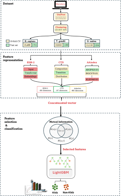
提出的框架利用先进的计算技术来预测KHIB位点。该框架结合了来自三个物种的数据集：H. Sapiens（人），，，，T.Gondii（寄生虫）， 和O. sativa（大米），分别有17,210、12,344和11,802肽序列。使用ESM-2嵌入，CTD描述符和AAINDEX衍生的物理化学特性提取特征。使用共同信息（MI）来增强特征选择的性能。LightGBM分类器用于区分Khib修饰的残基与非修饰的残基。流程图的示意图如图所示。 1。数据集从同行评审的出版物中策划了经过实验验证的KHIB站点，原始作者获得了适当的道德批准，机构审查委员会的许可，并根据其对三种进化多样的生物体的实验研究所需的知情同意：

H.Sapiensâ 

10，，，，30^{，，，，31，，，，T. Gondii 32和}O. sativa 33^，，，，34物种。^{对于每个生物体，从这些出版物中收集了KHIB修饰的位点及其相应的蛋白质登录数。最初的数据集包含25,676、17,594和14,079个实验验证的KHIB位点H. Sapiens}，，，，T. Gondii， 和O. sativa如表中所述，分别分布在多个组织/细胞类型中 1。表1用于KHIB站点预测的数据集中的样品分布。我们开发了一个Python，而不是检索完整的蛋白质序列 35

2^。该脚本利用了已发表研究的蛋白质登录数和特定的赖氨酸位置信息来查询Uniprot数据库，并及其周围的氨基酸提取靶赖氨酸。这种方法与基于质谱的PTM检测的典型工作流程一致，在分析前将蛋白消化成小肽。图2

通过系统评估程序确定肽提取的最佳窗口大小。

尽管PTM预测的窗口尺寸通常范围为35至39个氨基酸 ³⁶，由于KHIB站点已发布的预测因子数量有限，我们进行了优化实验。我们提取了窗户尺寸范围为35至47个氨基酸（即，每一侧中央赖氨酸两侧的23个残基）提取的肽，并使用该窗口长度评估了每个窗口长度的模型性能H. Sapiens由于其相对较大的样品，数据集作为代表性模型，其AUC平均超过10倍的交叉验证。

对于位于蛋白质末端附近的赖氨酸残基，侧翼残基不足，该符号被用作填充，以维持所有肽的均匀序列长度。如补充表中所示S1，43个残留窗口（中央赖氨酸的每一侧的21个残基）达到了最高的AUC，并被选为最佳窗口以进行进一步分析。

选择阴性样品（非Khib修饰的赖氨酸残基）对于PTM预测模型开发至关重要。我们没有检索完整的蛋白质序列，而是开发了一个Python脚本来直接提取肽序列。我们开发了一个Python脚本，该脚本使用登录号和已知的KHIB位置位置来从蛋白质中提取所有以赖氨酸为中心的肽，但不包括在报告的修饰位点的蛋白质。

与阳性样品相比，这种方法产生了大量的潜在负样本池。例如，在Hela细胞中H. Sapiens数据集，我们收集了6,544个阳性样品，而70,828个潜在的负样品。

为了解决固有的类不平衡，在保留生物学相关性的同时，按序列相似性聚集了阳性和负肽，然后随机选择负簇以匹配正簇的数量。这种基于聚类的平衡策略产生了最终数据集，并具有1：1的阳性比率，从而减轻了模型训练期间的类不平衡偏见。这种平衡方法与既定的PTM预测研究一致 ^{37，，，，38，，，，39}和KHIB预测研究 ⁶。

使用高标识（CD-HIT）工具的广泛建立的集群数据库实现了聚类步骤，以减少序列冗余并防止过度拟合。将共享超过40％序列相似性的序列分组为簇，其中一个代表性序列从每个集群中保留，以消除冗余训练示例。40％相似性阈值的选择是基于PTM预测研究的既定实践 ^{28，，，，40，，，，41}，在该阈值已被证明可以有效地平衡数据集多样性的同时，同时保持了足够的培训示例，以实现强大的模型性能。

这种聚类方法使用带有默认设置的CD-HIT应用于正肽和负肽集，除了相似性阈值设置为0.4，并且单词长度相应地调整为2。聚类后，原始的25,676个正面样本，来自原始的25,676个正样本。H. Sapiens减少到代表正簇的8,605。同样，T. Gondii和O. sativa数据集从17,594降低到5,901，分别从14,079个降低到6,172个正簇，证明了所有物种数据集的大量冗余清除。

负样本进行了相同的聚类过程。为了H. Sapiens，257,692个以赖氨酸为中心的负肽降低至31,052个簇。为了T. Gondii，62,201肽产生31,805个簇，用于O. sativa，将89,409肽降低至13,347个簇。从这些簇中，我们随机选择了相等数量的负簇以匹配正样品：8,605H. Sapiens，5,901T. Gondii和6,172O. sativa，分别产生17,210、11,802和12,344肽的最终平衡数据集。

为了使用统计严格的稳健模型开发和评估，每个物种特定的平衡数据集都被划分为训练（90％）和独立测试（10％）集。该数据分配策略可确保可靠的绩效估算，并防止过度适合可能损害模型概括的偏差。该训练集经过了10倍的交叉验证，以进行模型优化和超参数调整，这是一种统计重新采样技术，通过降低评估指标的差异来提供稳定的性能估计，并确保模型性能不取决于特定的训练测试测试分配比率。

独立的测试集仅用于最终绩效评估，作为无偏置的保留数据集，以评估真正的模型通用能力。该评估框架在计算生物学和机器学习中广泛接受，通过减少选择偏差和过度拟合来提供可靠的性能估计，从而提高了对报告的模型准确性的信心。

功能表示

特征表示（编码）是蛋白质序列分析的关键步骤，因为它将生物序列转化为与机器学习算法兼容的数值格式 ⁴²。编码策略的选择显着影响模型性能，因为这些策略捕获了生物学特性和模式的基础序列数据 ⁴³。为了优化预测精度，我们系统地评估了个人特征表示方法，包括Protbertâ ⁴⁴，word2vecâ ⁴⁵，单热编码和blosum62矩阵 ⁴⁶，以及ESM-2，CTD和AAINDEX功能。我们通过整合所有表示方法来增强预测性能，进一步探索了这些特征的组合。随后，我们采用了一种迭代消除策略，一次从合并设置中丢弃一种特征表示方法来评估其对性能的影响。该过程揭示了最大程度地促进模型准确性的功能的子集，因为丢弃残留功能不会降低性能。最终选定的功能集集成了来自ESM-2的进化见解，CTD的基于序列的模式以及来自AAINDEX描述符的理化属性。补充表中提供了替代特征表示方法的详细比较S2和图。S1。

基于嵌入的功能表示

ESM代表一种最新的基于变压器的蛋白质语言模型结构，旨在捕获蛋白质序列固有的进化，结构和功能特征 ⁴⁷。ESM-2模型采用了自我监督的学习范式，其中，变压器体系结构通过大规模蛋白质序列数据库中的掩盖语言建模来学习上下文化表示。具体而言，该模型取决于多头自我发项机制，这些机制能够同时建模蛋白质序列中局部残基相互作用和远距离依赖性，从而捕获短距离物理学特性和远距离的进化约束。 ⁴⁸。

ESM-2中的嵌入生成过程遵循分层方法，在该方法中，每个氨基酸位置首先转换为可学习的令牌嵌入，随后通过多个变压器层处理。每个变压器块由多头自发层组成，然后由位置馈电网络组成，始终应用残留连接和层归一化。自我发挥的机制计算所有残基对之间的注意力权重，从而使模型在为每个位置生成表示时都可以从整个序列中整合上下文信息。最后一个变压器层的最终隐藏状态用作上下文化的嵌入，同时编码局部氨基酸属性和全局序列上下文 ⁴⁹。

这项研究的模型选择涉及对具有不同参数尺度和嵌入维度的三种ESM-2变体的系统评估。ESM2_T6_8M_UR50D型号（800万（8亿）参数，6层，320维嵌入）的交叉验证AUC为0.757，而较大的ESM2_T30_150M_150M_UR_UR50D（150-M MODETERS，30层，30层，640-0-0-0-0-0-0-二维型）aucs a aucs a auc a a aucs and a and a a and a and a and aand99999999。中级ESM2_T12_35M_UR50D模型（35次参数，12层，480维嵌入）显示出改善的性能，AUC为0.762，代表了较小和较大的变体的改进。

观察到的性能模式反映了模型容量与特定任务优化之间的复杂关系。随着ESM-2模型中参数的数量的增加，嵌入维度扩大（320-480-640维度），从理论上讲，通过增强的特征空间复杂性提供了更有信息的蛋白质表示。但是，边际性能从最大模型相对于中间变体的增长并不能证明计算开销和内存需求的实质性增加是合理的。ESM2_T12_35M_UR50D变体的最佳性能表明，480维嵌入式捕获了足够的进化和结构信息，以实现KHIB预测任务，同时保持计算障碍性。

通过预训练的ESM2-35M模型处理每个肽序列，以生成残基级嵌入，其中每个氨基酸被表示为480维矢量，该矢量封装了多尺度生物学信息并捕获了必要的蛋白质序列。但是，在每个肽序列内的所有残基级嵌入中应用平均池聚集，以降低计算复杂性。由此产生的480维特征向量是KHIB预测管道的输入表示，最佳地平衡了生物学信息与计算效率。

基于序列的特征表示

组成，过渡和分布（CTD）特征，最初由杜布查克（Dubchak）等人引入。 ⁵⁰，在计算生物学中广泛使用用于编码蛋白质序列 ^{51，，，，52，，，，53}。这些特征通过捕获氨基酸的理化特性来提供序列级特性的结构化表示。CTD具有基于其物理化学属性（例如疏水性，电荷，极性和极化性）的定量氨基酸总体组成，过渡频率和空间分布。对于每个特性，将氨基酸分为三个预定义的类别，每个氨基酸均基于其组为1,2或3的指数编码。例如，就疏水性而言，氨基酸分组如下：第1组（极性）包括{r，k，e，d，d，q，n}；第2组（中性）包括{g，a，s，t，p，h，y};第3组（疏水）包括{C，L，V，I，M，F，W}。此分类框架对于计算CTD描述符至关重要，该描述符分为组成部分：组成，过渡和分布。

组成（C-CTD）： 组成描述符代表蛋白质序列中属于特定特性组的氨基酸的归一化频率。对于一系列长度 

\（\：l \），属性组的组成描述符\（\：我\）被计算为。

在哪里\（\：{n} _ {i} \）是组中的氨基酸的数量\（\：我\）， 和\（\：l \）是总序列长度。该描述符生成一个尺寸21的输出矢量，反映了七个氨基酸特性组和三种物理化学特性（例如疏水性，极性和极化性）的组合。

例如，考虑长度的序列{afdqfghiklmeprqtsiws} v\（\：l = 20 \）。使用基于疏水性的分组，每个组的计数如下：第1组占据6个位置，第2组占据7个位置，第3组在序列中占据了7个位置。相应的组成值计算为：

对于所有七个物理化学特性，重复此过程，导致大小为21的特征向量（7个属性â组）。

过渡（T-CTD）：描述符捕获了序列内不同组的氨基酸之间的过渡频率。当来自不同基团的氨基酸跟随某个组的氨基酸时，就会发生过渡。对于一对财产组\（我\）和\（J \），将过渡计算为：

在哪里\（\：l-1 \）代表可能长度序列的可能过渡的总数\（\：l \）。例如，在序列{afdqfghiklmeprqtsiws}中，基于组分配计数过渡。第1组和第2组之间有2个转变\（\：l-1 = 19 \），因此过渡频率是：

该计算是针对所有物理化学特性的三组的所有成对组合进行的，从而产生了21尺寸的特征向量。

分布（D-CTD）：描述符描述了整个序列中每组氨基酸的相对位置，重点是这些残基的空间扩散。它确定了第一个，第25个百分位，中位数（第50个百分位数），第75个百分位的位置，以及每组氨基酸的最后发生。对于一个小组\（我\），相对位置\（\：{p}^{th} \）出现的计算为。

在哪里\（\：p \）代表指定百分位数之一，\（\：l \）是序列长度。例如，按序列{afdqfghiklmeprqtsiws}和基于疏水性的分组，有7个残基属于第2组（中性），它们在序列中的位置为：1，6，6，7，13，13，16，16，17和20。\（\：（（（25/100）代表第二次发生的位置为6，残留物为6\（（（（（50/100）\ times 7 = 3.5 \ oft 4）\）\）代表第四次发生的位置为13，残留物为75％\（\：（（（75/100）代表第五次发生在位置16，最后一个残留物\（\：（（（100/100）\：\ times \：7 = 7）\）\）–代表第七次发生在位置20。因此，第2组的描述符为：

These calculations are repeated for all three groups and seven physicochemical properties, producing a total of (7 × 3 × 5) = 105 distribution features.

Property-based feature representation

The AAindex database ⁵⁴, a comprehensive repository comprising over 566 numerical indices, characterizes diverse physicochemical, biochemical, and structural properties of amino acids, constituting an invaluable resource for protein sequence analysis.In this study, 20 indices were selected for their established relevance to protein functionality, structural characteristics, and potential involvement in PTM mechanisms.These indices are enumerated in Supplementary TableS3。The selection process was guided by a systematic motif analysis of each species-specific dataset using the Two Sample Logo (Sect."Comparative motif analysis and position-specific amino acid preferences"), allowing for dataset-driven feature selection.

The distribution of key amino acid indices, hydrophobicity, residue volume, polarity, net charge, Electron-Ion Interaction Potential (EIIP), and information entropy across the 20 standard amino acids highlights their different contributions to amino acid properties.Hydrophobicity reflects the interaction of residues with the aqueous environment, playing a crucial role in protein folding and binding.Residue volume provides insights into steric effects within the protein structure, while polarity and net charge capture residue-specific interactions, such as hydrogen bonding and electrostatic effects, which are critical for determining the propensity of Khib sites.EIIP quantifies the electronic properties of amino acids, offering a window into their functional roles.Lastly, the entropy of information measures the variability and conservation of amino acids, shedding light on evolutionary constraints that shape sequence functionality.These indices collectively provide a comprehensive physicochemical and structural characterization essential for understanding the determinants of Khib modifications.

The encoding process maps each amino acid in a sequence to its corresponding numerical values for the selected 20 indices, generating a comprehensive numerical vector that preserves both residue-specific and positional information.This results in a feature vector of dimensions\(\:L\times20\)， 在哪里\(\:L\)denotes the sequence length.For sequences with\(\:L=43,\:\) the resulting feature vector has a dimensionality of 860. This approach ensured the retention of sequence-level and residue-specific characteristics, providing a rich representation of the physicochemical landscape for subsequent machine-learning tasks.

Complementary roles of hybrid features in modeling Khib modification mechanisms

This section highlights how integrating different feature types, namely evolutionary, compositional, and physicochemical, enhances the prediction of Khib sites by capturing complementary aspects of protein sequence information:

• ESM-2 evolutionary embeddings;trained on millions of diverse protein sequences from UniRef50 ⁵⁵, provide context-aware representations by leveraging transformer-based attention trained on large protein databases.They capture deep evolutionary conservation, non-local residue interactions, and implicit structural and domain information, enabling detection of complex enzymatic recognition patterns without relying on protein 3D structures ^{43，，，，56}。

• CTD descriptors capture local biochemical environments essential for enzymatic activity.Composition features reflect the abundance of amino acids with specific properties, supporting electrostatic interactions favourable for Khib catalysis.Transition and distribution descriptors highlight sequence boundary regions and spatial property distributions important for enzyme-substrate specificity.

• AAindex features encode experimentally-validated physicochemical properties (e.g., hydrophobicity, steric hindrance) of individual amino acids.Unlike CTD, which generalizes properties into broad categories, AAindex provides fine-grained, position-specific numeric values, offering precise biochemical insights into enzymatic recognition conditions.

Together, these hybrid features offer a multifaceted view of Khib modification mechanisms, with each contributing unique and complementary information on evolutionary context from ESM-2, biochemical composition from CTD, and physicochemical precision from AAindex, resulting in more accurate and biologically informed Khib site prediction.

Mutual information for feature selection

Mutual Information (MI) ⁵⁷was employed as the feature selection algorithm to enhance model performance and mitigate the risk of overfitting by identifying and prioritizing the most informative features ⁵⁸。MI quantifies the statistical dependency between two random variables by measuring the reduction in entropy of one variable given knowledge of the other ⁵⁹。This capability makes MI highly suitable for complex biological datasets, as it captures both linear and non-linear relationships between features and the target variable.Mathematically, MI for discrete random variables is expressed as:

在哪里\(\:X\)represents the feature variable,\(Y\)is the target variable,\(\:p(x,y)\)denotes their joint probability distribution and\(\:p\left(x\right)\)和\(\:p\left(y\right)\)are their respective marginal probability distribution.A higher value of\(\:I(x;y)\)indicates a stronger dependency between the feature and the target, highlighting its relevance for the classification task.

The choice of MI is based on experimental comparisons with alternative feature selection methods, each based on distinct mathematical principles.ANOVA, a filter-based method ⁶⁰, ranks features based on their statistical relationship with the target variable.Although computationally efficient, ANOVA assumes linear relationships and does not account for interactions or non-linear dependencies among features.Recursive Feature Elimination (RFE), a wrapper-based method ⁶¹, iteratively trains a model to eliminate the least important features, which allows it to account for feature interactions.However, RFE is computationally expensive, particularly for high-dimensional datasets like those used in this study.l₁regularization (Lasso) ⁶²and Elastic Net embedded methods ⁶³incorporate feature selection during model training by penalizing coefficients of less important features.

In comparison, MI, as a filter-based method, was found to offer distinct advantages in this study.Its ability to capture both linear and non-linear dependencies without requiring iterative model training made it computationally efficient, while still being robust in identifying biologically relevant features.Using the scikit-learn library, MI scores were computed for all features in the dataset to quantify their relevance to the classification of modified versus non-modified lysine residues.Features were ranked in descending order of their MI scores, ensuring that the most statistically informative features are prioritized.To reduce dimensionality while maintaining predictive performance, the top 700 features were selected based on their MI scores.These features provided a rich and concise representation of the dataset, serving as input to the LightGBM classifier for Khib site prediction.

Light gradient boosting machine (LightGBM)

LightGBM is a state-of-the-art gradient boosting framework developed by Microsoft  ⁶⁴, designed to address key limitations of traditional gradient boosting methods.It introduces several innovative techniques, such as histogram-based learning and Exclusive Feature Bundling (EFB), to enhance computational efficiency and scalability.Unlike conventional level-wise tree growth strategies, LightGBM employs a leaf-wise (best-first) tree growth strategy.This approach prioritizes splitting the leaf with the highest loss reduction, leading to deeper and more accurate trees while reducing training time and memory consumption.

The objective function of LightGBM is a combination of a loss function that measures how well the model fits the data and a regularization term to prevent overfitting by penalizing model complexity.At iteration\(\:t\), it can be expressed as:

在哪里\(\:N\)is the number of training samples,\(\:{y}_{i}\)is the true label for the\(\:ith\)样本，\(\:\hat{y}_{i}^{\left(t-1\right)}\)is the predicted value at iteration\(\:(t-1)\)，，，，\(\:{f}_{t}\left({x}_{i}\right)\)is the output of the newly added tree at iteration\(\:t\)，，，，\(\:l({y}_{i},\:\hat{y}_{i})\)is the binary cross-entropy (log loss) function and\(\:\varOmega\:({f}_{t})\)is the regularization term to control tree complexity, defined as:

在哪里\(\:T\)is the number of leaf nodes,\(\:{w}_{j}\)是\(\:jth\)leaf, γ is a parameter controlling the penalty for adding new leaf nodes, and λ is the\(\:{L}_{2}\)regularization term on leaf weights.

At each boosting iteration, LightGBM approximates the loss using a second-order Taylor expansion to enable efficient optimization:

在哪里\(\:{g}_{i}\)和\（\：{你好}\）are the first- and second-order gradients, and they are given by:

Compared to XGBoost ⁶⁵, LightGBM key strengths lie in its memory efficiency and training speed.While XGBoost employs a pre-sorted algorithm and stores all possible split points for continuous features, LightGBM implements histogram-based binning that discretizes continuous features into discrete bins.This optimization significantly reduces memory usage and computational complexity.Additionally, LightGBM Exclusive Feature Bundling (EFB) algorithm effectively manages sparse features by bundling mutually exclusive features, further reducing memory requirements without compromising model accuracy.

When compared to CatBoost ⁶⁶, LightGBM handles categorical features through a different approach.While CatBoost employs ordered target statistics with a permutation-based technique to prevent target leakage and reduce prediction shift, LightGBM depends on a special algorithm for categorical feature splitting based on Gradient-Based One-Sided Sampling (GOSS).GOSS retains instances with large gradients and random samples instances with small gradients, maintaining accuracy while improving training efficiency.However, the CatBoost ordered boosting approach may provide a more robust handling of categorical features in scenarios with high-cardinality categorical variables.

评估指标

To ensure a robust and reliable evaluation of the proposed framework, stratified 10-fold cross-validation  ⁶⁷被雇用。This method divides the dataset into 10 equally-sized folds, while preserving the original class distribution within each fold.During each iteration, nine folds were used for training, and the remaining fold was reserved for validation.This approach ensures that all samples are used for both training and validation across iterations.Furthermore, an independent test set comprising 10% of unseen data from each dataset was held out for final performance evaluation, providing an unbiased assessment of the model generalization capabilities to new data.

The model performance was evaluated using multiple complementary metrics derived from the confusion matrix, comprising True Positives (TP), True Negatives (TN), False Positives (fp), and False Negatives (fn）。The following metrics were computed:

Accuracy provides an overall measure of the model predictive correctness, while Sensitivity (also known as Recall in balanced binary classification tasks) is particularly important for capturing the proportion of true positive predictions, ensuring the model ability to identify key positive instances, which is crucial in biological applications like PTM prediction.Specificity gives the model ability to correctly identify negative samples, reducing false positives that could lead to erroneous biological inferences.The F1-Score balances Precision and Sensitivity, offering a harmonized metric suited for scenarios where both false negatives and false positives are of concern.Finally, the Matthews Correlation Coefficient (MCC) is a strong measure of how well the model performs overall.It is especially useful for checking the model reliability in binary classification tasks with balanced datasets, as in our experiments.

To further assess classification performance, Receiver Operating Characteristic (ROC) curves were generated by plotting the True Positive Rate (TPR) against the False Positive Rate (FPR) across varying decision thresholds ⁶⁸。Additionally, the AUC was calculated, offering a threshold-independent evaluation of the model discriminative power.An AUC value close to 1 indicates excellent discriminative ability, while values closer to 0.5 reveal random prediction.Comparative ROC analysis was conducted across all experimental configurations, enabling a quantitative evaluation of model performance and facilitating insight into the effectiveness of different feature encoding methods and classifiers.

Collectively, these evaluation protocols are reinforced by a comprehensive overfitting prevention strategy that ensures robust model generalization.This strategy includes (1) Dataset balancing and redundancy removal: balanced datasets with 1:1 positive-to-negative ratios prevent class imbalance bias, while CD-HIT clustering with 40% sequence similarity threshold eliminates redundant training examples that could lead to memorization rather than pattern learning;(2) Dimensionality optimization: mutual information-based feature selection reduces the risk of overfitting by retaining only the most informative features, while eliminating noise and irrelevant dimensions;(3) Rigorous data partitioning: the combination of stratified 10-fold cross-validation for model development and completely independent test sets (10% holdout) ensures unbiased performance assessment, with test data remaining entirely unseen during training and hyperparameter optimization;(4) Regularization optimization: LightGBMl1和l2regularization parameters are systematically optimized through Bayesian optimization using 100 Optuna trials, effectively balancing model complexity and generalization capacity._{结果与讨论}Hyperparameter optimizationThe LightGBM classifier for Khib site prediction requires systematic hyperparameter optimization to achieve optimal predictive performance._{This optimization was performed using OptunaÂ} 69

The optimization process was configured to maximize the AUC as the objective function, with a total of 100 trials executed to ensure a comprehensive exploration of the parameter space.

Optuna TPE algorithm iteratively refines hyperparameter selection through a probabilistic model that balances the exploration of unexplored regions with the exploitation of promising parameter combinations.^{This approach demonstrated convergence behaviour with optimal AUC values stabilizing after approximately 60–70 trials, indicating efficient parameter space exploration.}Table 

2lists the eight main hyperparameters we focused on: number of estimators (n_estimators), learning rate, maximum tree depth, number of leaves, feature subsampling ratio (colsample_bytree), data subsampling ratio (subsample), and minimum child samples.The parameter ranges were chosen following common LightGBM best practices.

The hyperparameter optimization yielded an improvement over default LightGBM settings, with the optimized configuration achieving an AUC improvement of approximately 4.2% compared to the baseline model.Convergence analysis revealed that the optimization process efficiently identified near-optimal parameter combinations, with minimal performance variance observed in the final 20 trials, confirming the robustness of the selected hyperparameters.

Comparative evaluation of feature representation methods on validation datasets

The development of an effective predictor for Khib sites using LightGBM necessitates a comprehensive evaluation of various feature representation methods to determine their discriminative capacity.This investigation comprises five distinct protein-encoding schemes that capture complementary aspects of protein sequences.The embedding-based scheme, ESM-2, leverages deep learning to extract contextual information from protein sequences.In contrast, the descriptors-based schemes, C-CTD, T-CTD, and D-CTD, encode sequence-level features that represent compositional, transitional, and distributional characteristics, respectively.The property-based scheme, AAindex, encodes intrinsic physicochemical properties of amino acids, providing insights into their biochemical attributes.

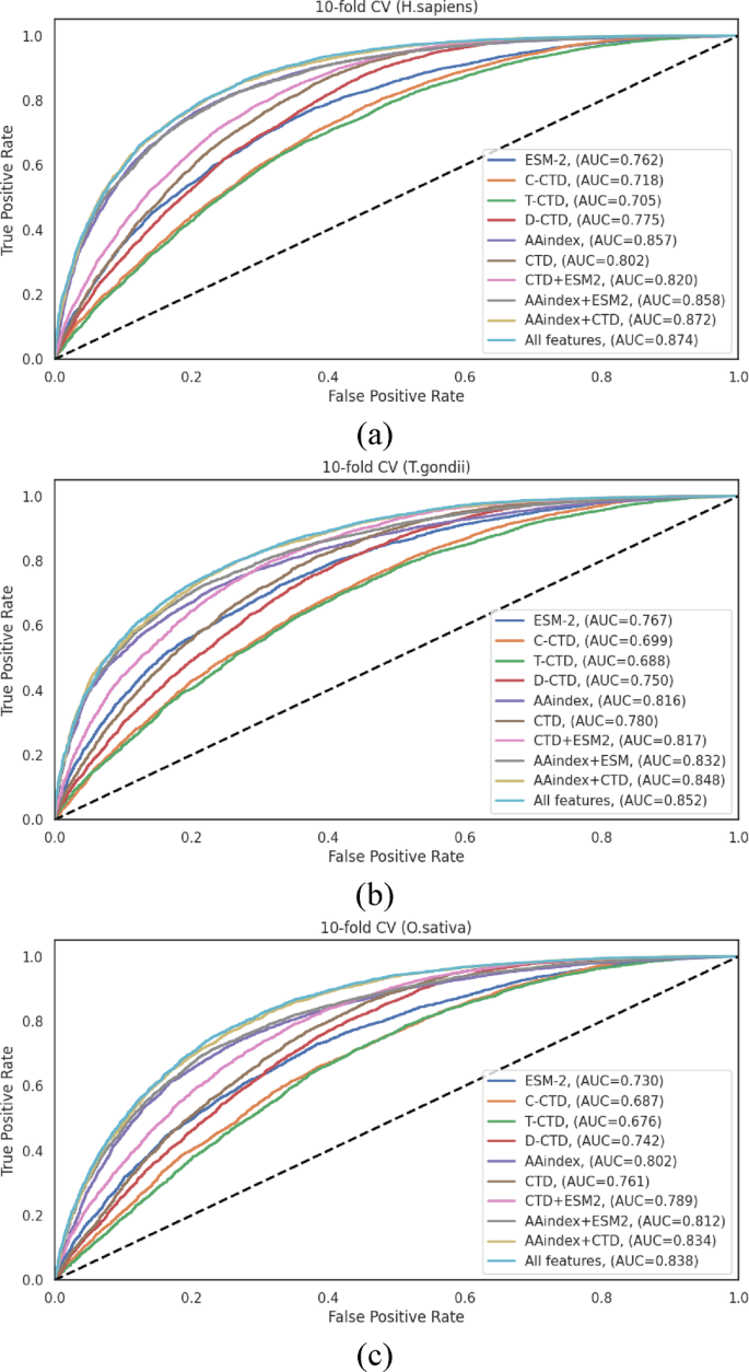
To maximize the feature space and enhance predictive performance, these encoding schemes were systematically integrated into hybrid feature sets, resulting in four additional combinations as detailed in TablesS4S6。These combinations include: (1) CTD, which integrates C-CTD, T-CTD, and D-CTD;(2) CTD + ESM;(3) AAindex + ESM;and (4) AAindex + CTD.Additionally, a comprehensive “All Features” set was created by integrating all five individual encoding methods.Performance assessment was conducted across three species-specific datasets (H. sapiens，，，，T. gondii， 和O. sativa) using stratified 10-fold cross-validation to ensure balanced class distributions.The performance metrics revealed distinct patterns across the datasets, with notable variations in the efficacy of different feature representation methods (TablesS4S6）。

在H. sapiensdataset (TableS4), the AAindex encoding method demonstrated excellent performance among individual representations, achieving an ACC of 0.780 and an AUC of 0.857.This performance significantly surpassed those of other individual methods (ESM, C-CTD, T-CTD, and D-CTD) by margins of 10.5% −19.82% for ACC and 10.58% −21.56% for AUC.The integration of AAindex with other encoding methods yielded statistically significant improvements.Specifically, the AAindex + CTD combination achieved an ACC of 0.790 and an AUC of 0.872, while the comprehensive “All Features” approach demonstrated the highest overall performance with an ACC of 0.791 and an AUC of 0.874.Notably, the MCC, a balanced measure of classification quality, reached 0.584 with the “All Features” approach, indicating robust discriminative capacity.

Analysis of theT. gondiidataset (TableS5) revealed that the AAindex encoding scheme again exhibited advanced performance among individual methods, with ACC and AUC values of 0.741 and 0.816, respectively.These values exceeded the average ACC and AUC of the other four individual encoding methods by 6.77% and 6.38%, respectively.Hybrid feature combinations demonstrated marked improvements, with the AAindex + CTD combination achieving an ACC of 0.764 and an AUC of 0.848.The “All Features” integration yielded the highest performance metrics (ACC of 0.766, and AUC of 0.852), ensuring that a comprehensive feature representation captures complementary aspects of the sequence information, effectively for this organism.

为了O. sativadataset (TableS6), the individual encoding methods demonstrated moderate performance, with AAindex again outperforming other individual methods (ACC of 0.735, and AUC of 0.802).The hybrid feature combinations showed incremental enhancements, with AAindex + CTD achieving an ACC of 0.755 and an AUC of 0.834.The “All Features” integration demonstrated the highest overall performance (ACC of 0.760, and AUC of 0.838), with a notable improvement in sensitivity (SN of 0.806) compared to individual methods.The MCC value of 0.522 for the “All Features” approach indicates notable improvement over individual encoding schemes, confirming the benefits of feature integration for this organism.

To validate the robustness of our approach and ensure that the observed patterns are not model-specific, parallel experiments were performed using Random Forest (RF), XGBoost, and CatBoost classifiers, with theH. sapiensdataset serving as a representative case.The supplementary material (TablesS7S9) presents these comparative results in detail.Importantly, all classifiers exhibited consistent patterns wherein hybrid feature representations enhanced performance across all evaluation metrics.However, LightGBM consistently demonstrated better efficacy compared to the alternative classifiers, affirming its particular suitability for this prediction task.

The performance differentials across feature representation methods, visualized through ROC curves in Fig. 3, clearly illustrate the advantages of hybrid approaches.The consistent pattern observed across all three species, where integrated feature sets outperformed individual encoding schemes, strongly ensures that different encoding methods capture complementary aspects of the sequence information, and their integration provides a more comprehensive representation of the characteristics relevant to Khib site prediction.

ROC curves of various feature representation methods on the 10-fold cross-validation data of (一个）H. sapiens, (b）T. gondii和 （c）O. sativa数据集。Comparative evaluation of feature representation methods on test sets

To evaluate the generalization ability of the LightGBM-based Khib prediction model, 10% of each species-specific dataset was reserved as an independent test set.

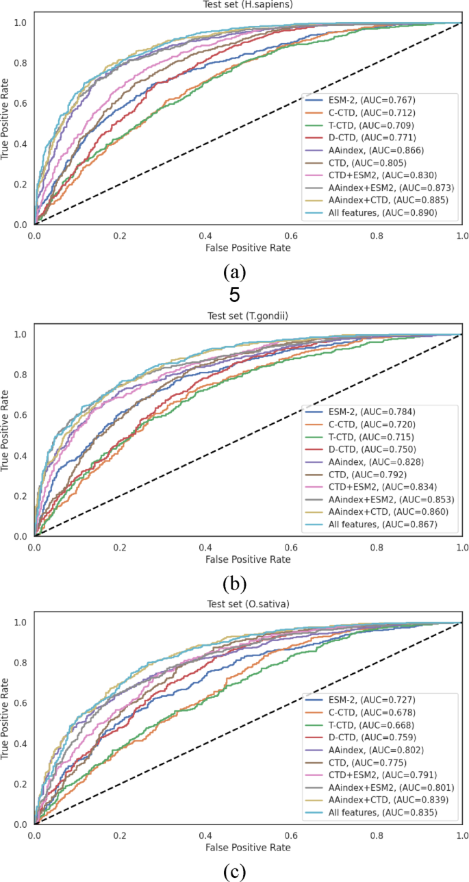
The model performance on these sets, using various encoding schemes and their combinations, closely aligned with the cross-validation results (Sec."Comparative evaluation of feature representation methods on validation datasets"). Notably, AAindex encoding demonstrated stable performance across all species achieving AUC scores of 0.866 (H. sapiens), 0.828 (T. gondii), and 0.802 (O. sativa) highlighting its strong and consistent discriminative power for Khib site prediction based on physicochemical properties.

The incremental integration of complementary feature representations yielded a progressive enhancement in predictive performance across all datasets.The initial combination of CTD descriptors established a foundational improvement over individual encoding.This performance was subsequently enhanced through the sequential integration of ESM-2 and AAindex features, culminating in the comprehensive “All Features” approach that consistently demonstrated good performance across all evaluation metrics.

在H. sapiensindependent test set (Table 3), the comprehensive feature integration (“All Features”) achieved the highest performance metrics: ACC = 0.814, SN = 0.840, SP = 0.787, F1-score = 0.821, MCC = 0.629, and AUC = 0.890.Notably, the AAindex + CTD combination also demonstrated robust performance (ACC = 0.808, and AUC = 0.885), revealing that these feature types capture complementary aspects of the sequence information, particularly relevant to Khib site prediction in human proteins.The performance differential between the best individual encoding (AAindex with ACC = 0.793, and AUC = 0.866) and the optimal feature combination (“All Features”) represented a statistically significant improvement of 2.65% in accuracy and 2.77% in AUC, underscoring the value of feature integration.

为了T. gondiiindependent test set (Table 4), the “All Features” approach similarly demonstrated enhanced performance, achieving ACC = 0.781, SN = 0.799, SP = 0.763, F1-score = 0.781, MCC = 0.562, and AUC = 0.867.The performance enhancement from the best individual encoding (AAindex with ACC = 0.756, and AUC = 0.828) to the optimal feature combination represented an improvement of 3.31% in accuracy and 4.71% in AUC.The AAindex + ESM combination also performed well (ACC = 0.773, and AUC = 0.853), showing that the integration of physicochemical properties with evolutionary information provides valuable discriminative features for this organism.

Analysis of theO. sativaindependent test set (Table 5) revealed that the “All Features” integration achieved the highest overall performance with ACC = 0.764, SN = 0.788, SP = 0.737, F1-score = 0.776, MCC = 0.526, and AUC = 0.835.Interestingly, the AAindex + CTD combination demonstrated comparable performance (ACC = 0.763, and AUC = 0.839).The performance improvement from the best individual encoding (AAindex with ACC = 0.728, and AUC = 0.802) to the optimal feature combination represented an enhancement of 4.95% in accuracy and 4.11% in AUC.

The ROC curves illustrated in Fig. 4visually represent the performance differentials across the various feature representation methods on the independent test sets.These curves provide clear evidence for the progressive enhancement in discriminative capacity achieved through feature integration, with the “All Features” approach consistently demonstrating the largest AUC across all datasets.

The steady improvement in performance from combining features, seen in both cross-validation and independent tests, shows that different encoding methods capture useful and complementary information about protein sequences for predicting Khib sites.The integration of these complementary features provides a more comprehensive representation of the sequence characteristics, enabling more accurate and robust prediction of Khib sites across diverse organisms.

ROC curves of various feature representation methods on the independent test sets of (一个）h。sapiens, (b) T. gondii和 （c）O. sativa数据集。Performance analysis of feature selection algorithms

The HyLightKhib framework has a comprehensive two-phase feature engineering strategy to optimize predictive performance.

The first phase focuses on integrating diverse feature representation techniques to capture complementary aspects of protein sequences.While this integration enhances discriminative capacity, it inherently introduces potential redundancy and noise that may impair computational efficiency and model generalization.Therefore, the second phase depends on feature selection algorithms to identify the most informative feature subset, with the primary objective of reducing computational overhead, while preserving model accuracy.

To identify the most effective dimensionality reduction approach, we systematically evaluated five established feature selection techniques: ANOVA, RFE, Lasso, Elastic Net, and MI.The evaluation was conducted across three species-specific datasets (H. sapiens，，，，T. gondii， 和O. sativa), with performance assessed through rigorous 10-fold cross-validation detailed in supplementary material TableS10, and independent test set validation TableS11。

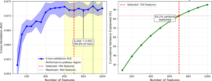
The original integrated feature set comprised 1,487 dimensions.Systematic evaluation acrossH. sapiensfeature subsets from 100 to 1,000 features revealed that performance plateaus beyond 600 features, with cross-validation AUC values remaining stable (0.872–0.873) across the 600–1000 feature range (Fig. 5）。While the maximum AUC (0.873) was achieved at 900 features, the performance difference from that obtained with 700 features was minimal (0.001 AUC units) and not statistically significant (p = 0.31).We selected 700 features as the optimal balance between performance and computational efficiency, as this threshold achieved 99.8% of the maximum performance level, while representing 83.2% of total mutual information variance.This leads to a reduction of the computational overhead by 22% compared to the case of 900 features.

Systematic optimization for mutual-information-based feature selection threshold.

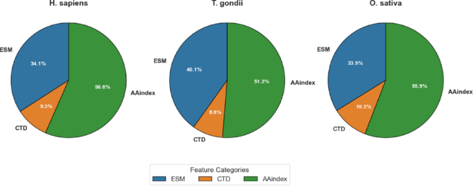
As detailed in Table 6, MI-based feature selection achieved balanced dimensionality reduction across all three feature categories (ESM, CTD, and AAindex), but with species-specific variations in the proportional representation of each category.为了H. sapiensdataset, the original 1,487 dimensions were reduced to 700, with proportional contributions of ESM (34.14%), CTD (9.29%), and AAindex (56.57%).这T. gondiidataset exhibited a slightly different distribution, with ESM features constituting a larger proportion (40.14%) compared toH. sapiens。CTD features maintained a similar contribution (8.57%), and AAindex features represented a somewhat smaller proportion (51.29%).为了O. sativadataset, the distribution more closely resembled that ofH. sapiens, with ESM, CTD, and AAindex features contributing 33.86%, 10.29%, and 55.86%, respectively.

These differential distributions, visualized in Fig. 6, provide valuable insights into the relative importance of different feature categories across species.The fact that a large share of AAindex features (51.29–56.57%) was chosen in all datasets highlights how important physicochemical properties are for predicting Khib sites.This matches the strong results AAindex gave when used alone, as shown in Sec."Comparative evaluation of feature representation methods on validation datasets" and "Comparative evaluation of feature representation methods on test sets". The varying contribution of ESM features, particularly the higher proportion inT. gondii(40.14%) compared to those ofH. sapiens(34.14%) andO. sativa(33.86%), reveals potential species-specific variations in the relevance of evolutionary information for Khib site prediction.

Elastic Net achieved more substantial dimensionality reductions through its inherent regularization mechanism, decreasing the feature dimensionality to 532, 446, and 447 forH. sapiens，，，，T. gondii， 和O. sativa， 分别。This more aggressive feature reduction did not consistently translate to advanced performance, highlighting the critical balance between dimensionality reduction and information preservation.

Visualization of feature category contribution after MI selection by dataset.

The performance metrics of the various feature selection methods on the independent test sets are comprehensively presented in TableS11。These results reveal several significant patterns and insights regarding the efficacy of feature selection in enhancing model performance.

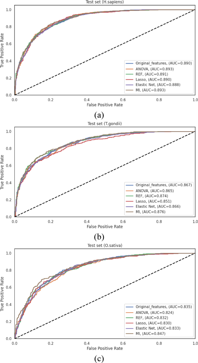
为了H. sapiensdataset, the original feature set established a robust baseline with an ACC of 0.814 and an AUC of 0.890.Among the feature selection methods, MI demonstrated effective performance, achieving comparable results with an ACC of 0.816 and an AUC of 0.893 while utilizing only 47% of the original features.ANOVA similarly achieved an AUC of 0.893, albeit with a slightly lower ACC of 0.801.The other methods maintained comparable performance levels, with Elastic Net showing modest improvement (ACC of 0.804 and AUC of 0.888) while achieving the most substantial dimensionality reduction.These results demonstrate that for theH. sapiensdataset, feature selection successfully maintains predictive performance while substantially reducing computational complexity.

Analysis of theT. gondiidataset revealed that the original feature set achieved an ACC of 0.781 and an AUC of 0.867.Both RFE and MI demonstrated enhanced discriminative capacity, with AUC values of 0.874 and 0.876, respectively. The MI achieved notable performance metrics (ACC of 0.782, MCC of 0.551 and AUC of 0.876) over the original feature set while reducing dimensionality.Lasso demonstrated the most conservative performance among the methods evaluated (ACC of 0.759, and AUC of 0.851), revealing that its aggressive sparsity-inducing mechanism may eliminate some informative features for this particular organism.Elastic Net, with its balanced regularization approach, achieved performance metrics (ACC of 0.782, AUC of 0.866) comparable to those of the original feature set while requiring substantially fewer features.

为了O. sativadataset, MI consistently achieved the highest performance among all evaluated methods, with an ACC of 0.765, an MCC of 0.517, and an AUC of 0.847.This performance represented an improvement over the original feature set (ACC of 0.764 and AUC of 0.835).The remaining feature selection methods demonstrated varying degrees of effectiveness, with ANOVA, RFE, and Elastic Net providing modest enhancements in specific metrics while maintaining an overall performance comparable to that of the original feature set.Lasso demonstrated the most substantial performance differential among the evaluated methods, achieving an ACC of 0.757 and an AUC of 0.829, ensuring potential species-specific variations in the effectiveness of sparsity-inducing feature selection.

The ROC curves illustrated in Fig. 7represent the performance differentials across the various feature selection methods for all three species datasets.These curves corroborate the quantitative metrics presented in TableS11, demonstrating the consistently notable performance of MI-based feature selection across all datasets.The comprehensive evaluation reveals that while the original feature set provides robust baseline performance, feature selection methods successfully maintain or enhance predictive performance while substantially reducing computational complexity.MI-based feature selection achieved the highest performance metrics across all three datasets while reducing feature dimensionality by approximately 47%, effectively capturing nonlinear relationships between features and class labels.

ROC curves illustrating the performance of LightGBM using different feature selection algorithms on the independent test sets of (一个）H. sapiens, (b）T. gondii， 和 （c）O. sativa数据集。Performance evaluation of machine learning classifiers

Having established the optimal feature representation approach and identified MI-based feature selection as the most effective dimensionality reduction technique, we evaluated the performance of various machine learning algorithms for Khib site prediction.

This comparative analysis encompassed seven widely-used classification algorithms: K-Nearest Neighbours (KNN) ⁷⁰, Adaptive Boosting (AdaBoost) ⁷¹, Random Forest (RF) ⁷², Support Vector Machine (SVM) ⁷³, XGBoost, CatBoost, and LightGBM.The evaluation was systematically conducted across the three species-specific datasets (H. sapiens，，，，T. gondii， 和O. sativa), utilizing the MI-selected feature subsets as input for each classifier.

To ensure a rigorous and fair comparison, each classifier hyperparameters were optimized through grid search cross-validation ⁷⁴。The final configurations were as follows: KNN was employed with the Euclidean distance metric withk = 9 neighbors;RF was based on the Gini impurity criterion for node splitting with an ensemble of 500 decision trees;AdaBoost was implemented with a learning rate of 1.0 and 500 weak learners;SVM was employed with a polynomial kernel function;XGBoost was configured with a learning rate of 0.1, maximum tree depth of 15, 500 estimators, and bothl₁和l₂regularization (λ = 1 and λ = 2, respectively);CatBoost was implemented with default hyperparameters and 500 iterations;and LightGBM was configured as detailed in Table 2。This systematic optimization strategy ensures that each algorithm performance was evaluated under optimal operating conditions.

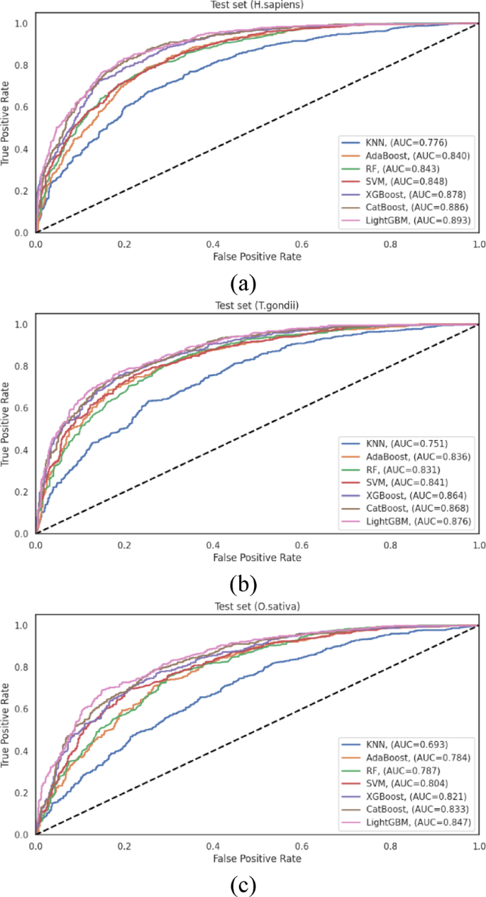
To ensure robust performance assessment, we implemented a dual validation strategy employing 10-fold cross-validation and independent test set evaluation.The cross-validation results are documented in TableS12。These results complement the independent test set evaluation presented in TableS13and visualized in Fig. 8, offering a more comprehensive assessment of classifier performance across diverse data scenarios.

为了H. sapiensdataset, LightGBM achieved the highest performance among all evaluated classifiers, with an ACC = 0.816 and an AUC = 0.893.CatBoost followed closely with ACC = 0.807 and AUC = 0.886, and XGBoost performed competitively with ACC = 0.793 and AUC = 0.878.The traditional algorithms, SVM, RF, and AdaBoost, exhibited moderate performance, with AUC values of 0.848, 0.843, and 0.840, respectively.KNN demonstrated substantially lower discriminative capacity (AUC = 0.776), showing that distance-based classification approaches may be less suitable for this prediction task.The performance differential between LightGBM and KNN (AUC difference of 0.117) underscores the significant impact of algorithm selection on predictive efficacy for human Khib sites.

Analysis of theT. gondiidataset revealed similar performance patterns, with LightGBM achieving the highest overall metrics (ACC = 0.782 and AUC = 0.876).CatBoost (AUC = 0.868) and XGBoost (AUC = 0.864) demonstrated comparable performance, indicating that gradient-boosting algorithms generally excel at capturing the complex patterns associated with Khib sites in this organism.SVM maintained competitive performance with AUC = 0.841, while RF and AdaBoost exhibited moderate discriminative capacity with AUC = 0.831, and 0.836, respectively.As observed in theH. sapiensdataset, KNN achieved notably lower performance with AUC = 0.751, providing further evidence of the limitations of distance-based approaches for this prediction task.

这O. sativadataset analysis reinforced the patterns observed in the other organisms, with LightGBM consistently achieving the highest performance among all classifiers with ACC = 0.765 and AUC = 0.847.CatBoost (AUC = 0.833) and XGBoost (AUC = 0.821) maintained their competitive performance, followed by SVM (AUC = 0.804).The ensemble-based approaches, RF and AdaBoost, demonstrated moderately lower performance with AUC = 0.787 and 0.784, respectively, while KNN exhibited the lowest discriminative capacity with AUC = 0.693.The substantial performance differential between LightGBM and KNN was most pronounced in this dataset, showing that the selection of an appropriate classification algorithm is particularly critical for plant Khib site prediction.

The consistent performance of LightGBM across all species datasets, validated by both cross-validation and independent testing, stems from its architectural strengths tailored to complex feature spaces like those in Khib site prediction.Its histogram-based binning enhances efficiency in handling high-dimensional data, while the leaf-wise tree growth with depth control captures complex nonlinear patterns without overfitting.Additionally, robust regularization contributes to its strong generalization ability.Although CatBoost and XGBoost also performed well, LightGBM consistently outperformed them, indicating that its specific design choices offer a distinct advantage for this classification task.

ROC curves showing the performance of different machine learning classifiers on the independent test sets of (一个）H. sapiens, (b）T. gondii和 （c）O. sativa数据集。Visualization of feature learning and cluster separation analysis

To evaluate HyLightKhib discriminative capacity,t

-distributed stochastic neighbor embedding (t-SNE)75was employed to visualize the feature transformation capabilities of the framework.The visualization analysis utilized the optimal configuration identified through a comprehensive performance evaluation, incorporating original input features with LightGBM classification following MI-based feature selection to maintain consistency with the best-performing model architecture.^这t

-SNE visualizations for the species-specificH. sapiens，，，，T. gondii， 和O. sativa datasets shown in Fig. 9demonstrate the effectiveness of our optimized framework in transforming the hybrid features into highly discriminative probability predictions.To provide a quantitative assessment beyond visual interpretation, silhouette scores and Davies-Bouldin indices were calculated for both the original feature space (left panels) and the LightGBM probability predictions (right panels).The silhouette score measures how similar data points are to their cluster compared to other clusters, with values ranging from − 1 to 1, where higher values indicate better-defined clusters.

Scores near 0 indicate overlapping clusters, while negative values indicate potential misclassification.The Davies-Bouldin index quantifies the average similarity between clusters, where lower values indicate better separation with more compact and well-separated clusters.Values closer to 0 represent optimal clustering quality.

为了H. sapiensdataset (Fig. 9a), the original feature space exhibited minimal class separation with a silhouette score of 0.008 and Davies-Bouldin index of 1.200, indicating substantial overlap between Khib-modified and non-modified lysine residues even after feature selection.The LightGBM probability predictions achieved substantial improvement with a silhouette score of 0.262 and the Davies-Bouldin index of 0.885.This improvement in silhouette score demonstrates the LightGBM ability to transform the original features into highly discriminative predictions.这

T. gondiidataset analysis (Fig. 9b) revealed the most pronounced discriminative transformation, with LightGBM probability predictions achieving a silhouette score of 0.285 and Davies-Bouldin index of 0.686 compared to those of the input features (silhouette score of 0.005, and Davies-Bouldin index of 1.100).This improvement in cluster separation metrics aligns with the 87.6% AUC performance reported in Sect. 3.5, demonstrating the LightGBM capacity to extract discriminative patterns from the optimally-selected feature subset for this organism.

为了O. sativadataset (Fig. 9c), the LightGBM transformed the input features into probability predictions with a silhouette score of 0.205 and Davies-Bouldin index of 0.831, representing an improvement over the input feature space (silhouette score of 0.006, and Davies-Bouldin index of 1.163).This improvement confirms the LightGBM effectiveness in processing the input feature set for plant protein analysis.

t-SNE visualization of input features (左边) and extracted predictions (正确的) by HyLightKhib of (一个）H. sapiens, (b）T. gondii和 （c）O. sativa数据集。

Comparative motif analysis and position-specific amino acid preferences

To further investigate the sequence characteristics underlying Khib site recognition and the varying classification performance across organisms, Two-Sample Logo analysis ⁷⁶was employed to identify position-specific amino acid preferences surrounding modification sites.The Two-Sample Logo is a statistical visualization tool that compares amino acid composition between two sequence sets (positive and negative samples) by calculating the difference in relative frequencies at each position and assessing statistical significance through hypothesis testing.

The Two-Sample Logo analysis was performed using a 43-residue window (−21 to + 21 positions relative to the central lysine) for all three species datasets.At each position, amino acid frequencies were compared between Khib-modified and non-modified sequences using a two-samplet-test with a significance threshold ofp-value ≤ 0.05.The resulting logos display amino acids with statistically significant differences in their occurrence frequencies between the two sample groups.

Enriched amino acids represent residues that occur more frequently in Khib-modified sequences compared to non-modified sequences at specific positions, showing positive associations with modification propensity.Conversely, depleted amino acids represent residues that occur less frequently in Khib-modified sequences, indicating negative associations with modification likelihood.The height of each letter is proportional to the magnitude of the frequency difference, with larger letters indicating more statistically significant and biologically relevant associations.

Two-sample logo analysis across three taxonomically diverse species reveals an evolutionary conservation of Khib recognition mechanisms alongside organism-specific adaptations.为了H. sapiens（图 10a), lysine (K) enrichment in upstream positions (−21 to −1) and glutamic acid (E) enrichment recommend cooperative recognition mechanisms within lysine-rich regions and favourable electrostatic environments for enzymatic machinery.Consistent proline (P) depletion indicates preferential modification in structured regions rather than helix-disrupted areas.

这T. gondiidataset (Fig. 10b) demonstrates conserved K enrichment patterns while exhibiting parasite-specific adaptations, including distinctive alanine (A) enrichment and reduced glutamic acid prominence compared to human sequences.Extensive serine (S) depletion (−8 to −10%) recommends spatial segregation mechanisms preventing phosphorylation-Khib crosstalk, while maintained proline depletion reinforces structured region preference.

Plant-specific adaptations inO. sativa（图 10c) maintain core recognition features with pronounced E enrichment exceedingT. gondiilevels, indicating enhanced acidic residue requirements in plant Khib systems.Unique arginine (R) depletion patterns (−6 to −8%) alongside consistent proline reduction recommend the avoidance of excessive positive charge density and structural disruptions.

Quantitative analysis reveals hierarchical motif signatures correlating directly with computational performance.Maximum lysine enrichment decreases acrossH. sapiens(14.5%),T. gondii(13.5%), andO. sativa(12.7%), corresponding precisely to classification performance with 89.3%, 87.6%, and 84.7% AUC, respectively.

Comparison of the amino acid preferences near the Khib sites in the (一个）H. sapiens, (b）T. gondii和 （c）O. sativa数据集。Comparative analysis with state-of-the-art Khib prediction methods

To evaluate the performance of the HyLightKhib model in identifying Khib sites, its results were compared with those of existing Khib prediction tools: iLys-Khib, KhibPred, DeepKhib and ResNetKhib.

iLys-Khib used a 35-residue window centred on the lysine and a fuzzy SVM.This approach reduces noise by giving different weights (fuzzy memberships) to samples depending on how relevant they are and how close they are to the class center.It incorporates three feature encoding methods: Amino Acid Factors (AAF), Binary Encoding (BE), and the Composition ofk-spaced Amino Acid Pairs (CKSAAP) to capture the sequence context surrounding Khib sites.Feature selection used the maximum Relevance Minimum Redundancy (mRMR) method to retain the most informative features.

KhibPred used the same feature encoding as iLys-Khib but with a smaller window size of 29. It also used an ensemble SVM classifier to handle the imbalance in the dataset, where Khib sites are fewer than non-Khib sites.To handle this issue, the negative samples were divided into seven subsets, with an individual SVM trained on each subset, then combined with the positive samples.The ensemble model aggregated the predictions from all SVMs to make the final classification.

DeepKhib is a deep learning framework that employs a CNN architecture with a one-hot encoding approach.The model utilizes a four-layer architecture consisting of an input layer with one-hot encoding representation, a convolution layer containing four convolution sublayers (with 128 filters each of lengths 1, 3, 9, and 10) and two max pooling sublayers, a fully-connected layer incorporating global average pooling to prevent overfitting, and an output layer with sigmoid activation function for probability scoring.

ResNetKhib is the first cell-type-specific deep learning predictor for lysine Khib sites, employing a residual neural network (ResNet) architecture with a one-dimensional convolution and transfer learning strategy across different cell types and species.The model architecture consists of five key components: an input layer, an embedding layer, a convolution module containing six blocks with residual connections (first block with 64 filters, followed by five residual blocks), a fully-connected layer with 16 neurons for feature flattening, and an output layer with sigmoid activation for probability scoring.Both DeepKhib and ResNetKhib have 37-residue windows.

For a comprehensive methodological comparison, the SVM models documented in the iLys-Khib and KhibPred publications ^{25，，，，26}and the CNN architectures described in DeepKhib and ResNetKhib ^{6，，，，28}were reimplemented according to their original specifications.These models were subsequently trained and evaluated using our curated datasets under identical experimental conditions as our proposed method, thereby ensuring a fair and direct comparison.This approach eliminates potential confounding variables that might arise from differences in data preprocessing, partitioning strategies, or evaluation metrics.

Model training was performed using consistent cross-validation protocols across all compared methods, and performance was assessed on the same independent test sets to provide an unbiased evaluation of predictive capabilities.The comparative evaluation results across all benchmark methods are presented in TableS14。

As shown in TableS14, HyLightKhib achieved accuracy improvements of approximately 16.1%, 15.5%, 6.1%, and 2.9% over iLys-Khib, KhibPred, DeepKhib, and ResNetKhib, respectively, for theH. sapiens数据集。The improvements for theT. gondiidataset were 9.5%, 8.9%, 1.3%, and 0.6% compared to the same methods.为了O. sativadataset, HyLightKhib achieved accuracy improvements of 13.8%, 11.35%, 8.7%, and 4.8% compared to the aforementioned predictors.

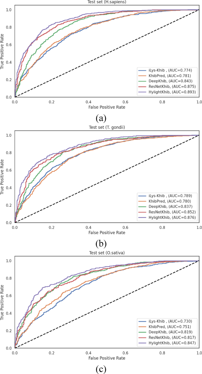
The ROC curves and the corresponding AUC values presented in Fig. 11reveal more modest improvements, particularly compared to recent deep learning methods.HyLightKhib achieved AUC values of 0.893, 0.876, and 0.847 forH. sapiens，，，，T. gondii， 和O. sativa， 分别。When compared to ResNetKhib, the most competitive baseline method, the AUC improvements were 1.8%, 2.4%, and 3.0% for the three datasets, respectively.

ROC curves comparing existing Khib predictors and HyLightKhib on the independent test sets for (一个）H. sapiens, (b）T. gondii， 和 （c）O. sativa数据集。The statistical significance of AUC differences was assessed using the Hanley & McNeil method 

77^{for comparing correlated ROC curves derived from identical test sets.}Although newer methods such as DeLong’s ⁷⁸test are now common, Hanley & McNeil remains a valid approach for estimating the significance of AUC differences in diagnostic and predictive modeling.Using this method, HyLightKhib demonstrated highly-significant improvements (p < 0.001) in overall existing predictors across the three species datasets, providing robust statistical evidence for its superior performance.For the H. sapiens dataset, significant improvements were observed over ResNetKhib (p

 = 7.47 × 10⁻¹¹), DeepKhib (p < 10⁻¹⁶), iLys-Khib (p < 10⁻¹⁶), and KhibPred (p < 10⁻¹⁶).Similarly, theT. gondiidataset showed highly significant improvements over ResNetKhib (p = 6.11 × 10⁻¹⁰), DeepKhib (p < 10⁻¹⁶), iLys-Khib (p < 10⁻¹⁶), and KhibPred (p < 10⁻¹⁶).这O. sativadataset exhibited the same pattern with significant improvements over ResNetKhib (p = 8.23 × 10⁻¹²), DeepKhib (p < 10⁻¹⁶), iLys-Khib (p < 10⁻¹⁶), and KhibPred (p < 10⁻¹⁶).However, the primary advantage of HyLightKhib lies in its computational efficiency rather than dramatic performance gains.A comprehensive computational efficiency analysis was conducted to quantitatively assess the practical applicability of HyLightKhib compared to existing models.All experiments were performed on a standard desktop system (AMD Ryzen 5 7520U, 2.80 GHz, and 16.0 GB RAM).As detailed in Table 7, HyLightKhib demonstrates computational advantages across all evaluated metrics.HyLightKhib demonstrated enhanced computational efficiency across all three datasets, with training times of 19.95, 19.36, and 21.77 seconds for the

H. sapiens，，，，T. gondii， 和

O. sativadatasets, respectively.When compared to existing methods, HyLightKhib achieved substantial training speedups: 92-166 times faster than DeepKhib (1994.11–3321.92 seconds), 19-27 times faster than ResNetKhib (414.59–548.05 seconds), 347-528 times faster than KhibPred (7236.3–10541.27 seconds), and 16–40 times faster than iLys-Khib (311.69–793.69 seconds).The most pronounced efficiency gains were observed against the ensemble-based KhibPred, highlighting HyLightKhib’s streamlined architecture.Memory utilization analysis revealed HyLightKhib resource-efficient design, with peak consumption ranging from only 1.61–6.10 megabytes (MB) across all datasets.This represents substantial memory reductions compared to all baseline methods: 33-127 times less than DeepKhib (73.79-378.34 MB), 49-75 times less than ResNetKhib (121.07-298.23 MB), 42-109 times less than KhibPred (174.9-254.77 MB), and 10-121 times less than

iLys-Khib (50.21–194.00 MB).The minimal memory footprint makes HyLightKhib particularly suitable for deployment in resource-constrained environments.

Inference performance evaluation demonstrated HyLightKhib capability for high-throughput applications, processing individual samples in 0.021–0.046 seconds across all datasets.This translates to significant inference accelerations: 63-132 times faster than DeepKhib (2.51–3.84 seconds), 24-48 times faster than ResNetKhib (1.014–1.29 seconds), 131-433 times faster than iLys-Khib (5.31–12.57 seconds), and remarkably 2139-4677 times faster than KhibPred (98.21–99.74 seconds).These performance metrics underscore HyLightKhib practical advantage for large-scale proteome-wide Khib site prediction tasks.

These quantitative computational benchmarks provide compelling empirical evidence for practical advantages in real-world applications.The significant reduction in computational resources, while maintaining competitive accuracy, makes HyLightKhib particularly suitable for large-scale proteomic analyses and integration into high-throughput experimental workflows.This empirical evaluation demonstrates that HyLightKhib offers an optimal balance between predictive performance and computational efficiency.

This study introduced HyLightKhib, a computational framework operating on 43-residue peptide sequences for predicting Khib sites by integrating ESM-2 embeddings, CTD descriptors, and selected amino acid physicochemical properties with mutual information-based feature selection and LightGBM classification.Comprehensive benchmarking acrosshuman ，，，，parasite ， 和rice proteomes revealed accuracy improvements ranging from 2.9 to 16.1% compared to existing tools, with more modest AUC improvements of 1.8-3.0% over the most competitive baseline methods.The primary contribution lies in computational efficiency, achieving 16-528 times faster training, 10-127 times lower memory consumption, and 24-4677 times higher inference speeds compared to deep learning alternatives, making the framework particularly suitable for high-throughput experimental workflows while maintaining competitive predictive accuracy.

Despite these advancements, several limitations must be acknowledged.The generalizability of the model to species beyond the three organisms tested remains uncertain.The current design does not incorporate three-dimensional structural information or consider potential crosstalk with other PTMs, both of which may influence site accessibility and biological function.Furthermore, the model was trained on an artificially balanced dataset, which may not reflect the true prevalence of Khib sites in vivo.Lastly, experimental validation of the predicted Khib sites remains essential to confirm their biological relevance and practical utility.

Looking ahead, future work should focus on extending the framework to additional species, integrating structural and multi-PTM information, and validating predictions through experimental assays.Nevertheless, HyLightKhib has several real-life applications in both biomedical and biotechnological research.It facilitates the investigation of epigenetic regulation and protein function by identifying candidate Khib sites, which are involved in key biological processes such as gene expression and chromatin remodeling.These insights can aid in the discovery of disease-associated biomarkers, guide experimental validation by prioritizing modification sites, and support therapeutic target identification.In addition, the framework can be applied to plant and microbial systems to enhance crop improvement and pathogen control, making it a valuable tool for advancing both healthcare and agricultural biotechnology.The framework computational scalability democratizes access to PTM prediction tools across research institutions with diverse resources, contributing to a deeper understanding of Khib modifications while promoting a balance between predictive accuracy and operational efficiency.