Characterizing privacy in quantum machine learning

General Framework

Variational quantum circuits for machine learning

A variational quantum circuit (VQC) is described in the following manner. We consider the d-dimensional input vector \({\bf{x}}\in {\mathcal{X}}\subset {{\mathbb{R}}}^{d}\), which is loaded into the quantum encoding circuit V(x) of n qubits to produce a feature map with the input state mapping,

This operation loads the input vector of dimension d to a Hilbert space \({\mathcal{H}}={({{\mathbb{C}}}^{2})}^{\otimes n}\) of dimension dim(ρ(x)) = 2ⁿ. We will explicitly consider the scenario where n = Θ(d), which is a common setting in most existing VQC algorithms, and hence the number of qubits in a given algorithm will be of the same order as the input vector dimension d. The state ρ(x) is then passed through a variational circuit ansatz U(θ) defined as

which is parameterized by a vector of variational parameters θ = [θ₁, ⋯ , θ_D], where D is the total number of variational parameters. Here {H₁, ⋯ , H_N} are the set of N Hermitian generators of the circuit U. The generator assignment map ν: [D] → [N] is used to assign one the generator H_ν(k) to the corresponding variational parameter θ_k. Under this notation, multiple distinct variational parameters can use the same generator. This is the case for repeated layers of a variational ansatz, where for L repeated layers, one would have D = NL and ν(k) = ((k − 1)mod N) + 1. We note that the above structure is quite general since some common ansatz structures such as the hardware efficient ansatz, the quantum alternating operator ansatz, and Hamiltonian variational ansatz, among others, are all encapsulated in this framework as highlighted in ref. ³⁹.

The parameterized state ρ(x) is passed through a variational circuit denoted by U(θ), followed by the measurement of some observable \({\bf{O}}\in {\mathcal{H}}\). For a given θ, the output of the variational quantum circuit model is expressed as the expectation value of O with the parameterized state,

For the task of optimizing the variational quantum circuits, the model output is fed into the desired cost function Cost(θ, x), which is subsequently minimized to obtain,

where θ^* are the final parameter values after optimization. Typical examples of cost functions include cross-entropy loss, and mean-squared error loss, among others⁴⁰.

The typical optimization procedure involves computing the gradient of the cost function with respect to the parameters θ, which in turn, involves computing the gradient with respect to the model output y_θ(x)

Going forward, we will directly deal with the recoverability of input x given C_j, instead of working with specific cost functions. Details of how to reconstruct our results when considering gradients with respect to specific cost functions are covered in the Supplementary file Sec II.

Lie theoretic framework

We review some introductory as well as recent results on Lie theoretic framework for variational quantum circuits which are relevant to our work. For a more detailed review of this topic, we refer the reader to^39,41. We provide the Lie theoretic definitions for a periodic ansatz of the form Eq. (2).

Definition 1

(Dynamical Lie Algebra). The dynamical Lie algebra (DLA) \({\mathfrak{g}}\) for an ansatz U(θ) of the form Eq. (2) is defined as the real span of the Lie closure of the generators of U

where the closure is defined under taking all possible nested commutators of S = {iH₁, ⋯ , iH_N}. In other words, it is the set of elements obtained by taking the commutation between elements of S until no further linearly independent elements are obtained.

Definition 2

(Dynamical Lie Group). The dynamical Lie group \({\mathcal{G}}\) for an ansatz U(θ) of the form of Eq. (2) is determined by the DLA \({\mathfrak{g}}\) such that,

where \({e}^{{\mathfrak{g}}}:= \{{e}^{i{\bf{H}}},i{\bf{H}}\in {\mathfrak{g}}\}\) and is a subgroup of SU(2ⁿ). For generators in \({\mathfrak{g}}\), the set of all U(θ) of the form Eq (2) generates a dense subgroup of \({\mathcal{G}}\).

Definition 3

(Adjoint representation). The Lie algebra adjoint representation is the following linear action: \(\forall {\bf{K}},{\bf{H}}\in {\mathfrak{g}}\),

and the Lie group adjoint representation is the following linear action \(\forall {\bf{U}}\in {\mathcal{G}},\forall {\bf{H}}\in {\mathfrak{g}}\),

Definition 4

(DLA basis). The basis of the DLA is denoted as \({\{i{{\bf{B}}}_{\alpha }\}}_{\alpha }\), \(\alpha \in \{1,\cdots \,,\,\text{dim}\,({\mathfrak{g}})\}\), where B_α are Hermitian operators and form an orthonormal basis of \({\mathfrak{g}}\) with respect to the Frobenius inner product.

Any observable O is said to be entirely supported by the DLA whenever \(i{\bf{O}}\in {\mathfrak{g}}\), or in other words

where μ_α is the coefficient of support of O in the basis B_α.

Definition 5

(Lie Algebra Supported Ansatz³⁶). A Lie Algebra Supported Ansatz (LASA) is a periodic ansatz of the form Eq. (2) of a VQC where the measurement operator O is completely supported by the DLA \({\mathfrak{g}}\) associated with the generators of U(θ), that is,

In addition to its connections to the trainability of a VQC, this condition also implies that \(\forall {\boldsymbol{\theta }},{U}^{\dagger }({\boldsymbol{\theta }})i{\boldsymbol{O}}U({\boldsymbol{\theta }})\in {\mathfrak{g}}\), which enables us to express the evolution of the observable O in terms of elements of \({\mathfrak{g}}\). This is key to some simulation algorithms that are possible for polynomial-sized DLAs^37,38.

Input recoverability definitions

In this section, we provide meaningful definitions of what it means to recover the classical input data given access to the gradients \({\{{C}_{j}\}}_{j = 1}^{D}\) of a VQC. Notably, our definitions are motivated in a manner that allows us to consider the encoding and variational portions of a quantum variational model separately.

A useful concept in machine learning is the creation of data snapshots. These snapshots are compact and efficient representations of the input data’s feature map encoding. Essentially, a snapshot retains enough information to substitute for the full feature map encoded data, enabling the training of a machine learning model for a distinct task with the same data but without the need to explicitly know the input data was passed through the feature map. For example, in methods such as \({\mathfrak{g}}\)-sim³⁸, these snapshots are used as input vectors for classical simulators. The simulator can then process these vectors efficiently under certain conditions, recreating the operation of a variational quantum circuit.

It will become useful to classify the process of input data x recovery into two stages; the first concerns recovering snapshots of the quantum state ρ(x) (Eq (1)) from the gradients, which involves only considering the variational part of the circuit.

Definition 6

(Snapshot Recovery). Given the gradients C_j, j ∈ [D] as defined in Eq (5) as well as the parameters θ = [θ₁, ⋯ , θ_D], we consider a VQC to be snapshot recoverable if there exists an efficient \({\mathcal{O}}(poly(d,\frac{1}{\epsilon }))\) classical polynomial time algorithm to recover the vector e_snap such that,

for some {B_α} forming a Frobenius-orthonormal basis of the DLA \({\mathfrak{g}}\) corresponding to U(θ) in Eq. (2), and the above holds for any ϵ > 0. We call e_snap the snapshot of x.

In other words, e_snap is the orthogonal projection of the input state ρ(x) onto the DLA of the ansatz, and thus the elements of e_snap are the only components of the input state that contribute to the generation of the model output y_θ(x) as defined in Eq. (3). Here, we constitute the retrieval of the snapshot e_snap of a quantum state ρ(x) as weak privacy breach, since the snapshot could be used to train the VQC model for other learning tasks involving the same data {x} but without the need to use the actual data. As an example, consider an adversary that has access to the snapshots corresponding to the data of certain customers. Their task is to train the VQC to learn the distinct behavioral patterns of the customers. It becomes apparent that the adversary can easily carry out this task without ever needing the original data input since the entire contribution of the input x in the VQC output decision-making y_θ(x) is captured by e_snap.

Next, we consider the stronger notion of privacy breach in which the input data x must be fully reconstructed. Assuming that the snapshot has been recovered, the second step we therefore consider is inverting the recovered snapshot e_snap to find the original data x, a process that is primarily dependent on the encoding part of the circuit. Within our snapshot inversion definition, we consider two cases that enable different solution strategies: snapshot inversion utilizing purely classical methods and snapshot inversion methods that can utilize quantum samples.

Definition 7

(Classically Snapshot Invertible Model). Given the snapshot e_snap as the expectation values of the input state ρ(x), we say that VQC admits classical snapshot invertibility if there exists an efficient \({\mathcal{O}}(\,\text{poly}\,(d,\frac{1}{\epsilon }))\) polynomial time classical randomized algorithm to recover

with probability at least \(p=\frac{2}{3}\), for any user defined ϵ > 0.

Definition 8

(Quantum Assisted Snapshot inversion). Given the snapshot e_snap as the expectation values of the input state ρ(x), and the ability to query \(\,\text{poly}\,(d,\frac{1}{\epsilon })\) number of samples from the encoding circuit V to generate snapshots \({{\bf{e}}}_{{\rm{snap}}}^{{\prime} }\) for any given input \({{\bf{x}}}^{{\prime} }\), we say that VQC admits quantum-assisted snapshot invertibility, if there exists an efficient \({\mathcal{O}}(\,\text{poly}\,(d,\frac{1}{\epsilon }))\) polynomial time classical randomized algorithm to recover

with probability at least \(p=\frac{2}{3}\), for any user defined ϵ > 0.

In this work, we specifically focus on input recoverability by considering the conditions under which VQC would admit snapshot recovery followed by snapshot invertibility. Considering these two steps individually allows us to delineate the exact mechanisms that contribute to the overall recovery of the input.

It is important to mention that it may potentially only be possible to recover the inputs of a VQC up to some periodicity, such that there only exists a classical polynomial time algorithm to recover \(\tilde{{\bf{x}}}={\bf{x}}+{\bf{k}}\pi\) up to ϵ-closeness, where \({\bf{k}}\in {\mathbb{Z}}\). As the encodings generated by quantum feature maps inherently contain trigonometric terms, in the most general case it may therefore only be possible to recover x up to some periodicity. However, this can be relaxed if the quantum feature map is assumed to be injective.

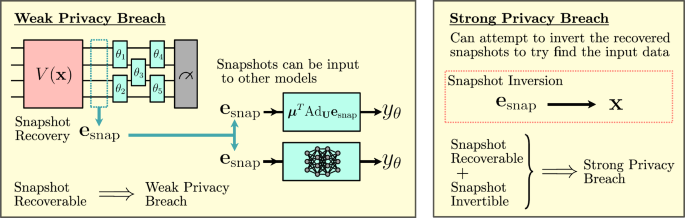
Figure 2 shows a diagram that highlights the Lie algebraic simulation method³⁸ along with specifications of the input recovery framework as defined in this work.

a Visualization of the difference between the circuit implementation of a variational quantum model and a Lie algebraic simulation procedure of the same model³⁸. In the Lie algebraic Simulation framework³⁸, input data x is encoded into a quantum circuit using V(x), however, the measurements are then performed on this encoded state and used to form a vector of snapshot expectation values. This vector of snapshot expectation values can then be passed as inputs to a classical simulator that uses the adjoint form of U(θ), which can be performed with resources scaling with the dimension of the DLA formed by the generators of U(θ). b In this work, we assess the ability to recover an input x from gradients C_j. This can be broken into two parts: Firstly, the snapshot e_snap must be recovered from the gradients C_j, which corresponds to reversing the Lie algebraic simulation step. Secondly, the recovered snapshot e_snap must be inverted to find the original data x, which requires finding the values of x that when input into V(x) will give the same snapshot values e_snap. If both snapshot recovery and snapshot inversion can be performed, then it admits efficient input recovery.

Snapshot recovery

This section addresses the weak privacy notion of recovering the snapshots of the input as introduced in Def 6. As the name implies, the goal here is to recover the vector e_snap for some Schmidt orthonormal basis \({\{{{\bf{B}}}_{\alpha }\}}_{\alpha \in \text{dim}({\mathfrak{g}})}\) of the DLA corresponding to the VQC ansatz U(θ), given that the attacker is provided the following information,

1. 1.

   D gradient information updates \({C}_{j}=\frac{\partial {y}_{{\boldsymbol{\theta }}}({\bf{x}})}{\partial {\theta }_{j}},j\in [D]\) as defined in Eq. (5).

2. 2.

   Ansatz architecture U(θ) presented as an ordered sequence of Hermitian generators \({\{{\theta }_{k},{{\bf{H}}}_{\nu (k)}\}}_{k = 1}^{D}\), where H_ν(k) is expressed as a polynomial (in the number of qubits) linear combination of Pauli strings.

3. 3.

   Measurement operator O, which satisfies the LASA condition according to Def 5 and is expressed as a polynomial (in the number of qubits) linear combination of Pauli strings

Recovering these snapshots will enable an attacker to train the VQC model for other learning tasks that effectively extract the same information from the input states ρ(x) but without the need to use the actual data. The main component of the snapshot recoverability algorithm makes use of the \({\mathfrak{g}}\)-sim^37,38 framework, which we briefly review in the following subsection while also clarifying some previously implicit assumptions, to construct a system of linear equations that can be solved to recover e_snap as detailed in Algorithm 2.

Review of Lie-algebraic simulation framework

We start by reviewing the \({\mathfrak{g}}\)-sim framework^37,38 for classically computing the cost function and gradients of VQCs, when the observable lies in the DLA of the chosen ansatz. Specifically, this framework evolves the expectation values of observables via the adjoint representation. However, a necessary condition for this procedure to be efficient is that the dimension of the DLA (\(\,\text{dim}\,({\mathfrak{g}})\)) is only polynomially growing in the number of qubits.

The first step of \({\mathfrak{g}}\)-sim consists of building an orthonormal basis for the DLA \({\mathfrak{g}}\) given \({(\{{\theta }_{k},{{\bf{H}}}_{\nu (k)}\})}_{k = 1}^{D}\). Algorithm 1 presents a well-known procedure to do this. The procedure simply computes pairwise commutators until no new linearly independent elements are found. Given that all operators are expressed in the Pauli basis, the required orthogonal projectors and norm computations performed by Algorithm 1 can be performed efficiently. If the dimension of DLA is \({\mathcal{O}}(\,\text{poly}\,(n))\), then the iteration complexity, i.e., the number of sets of commutators that we compute, of this procedure is polynomial in n. However, an important caveat is that potentially the elements forming our estimation for the DLA basis could have exponential support on the Pauli basis, which is a result of computing new pairwise commutators at each iteration. Thus, for this overall procedure to be efficient, we effectively require that the nested commutators of the generators H_k do not have exponential support on the Pauli basis.

Definition 9

(Slow Pauli Expansion). A set of Hermitian generators {H₁, …, H_N} on n-qubits expressed as linear combinations of \({\mathcal{O}}(\,\text{poly}\,(\dim ({\mathfrak{g}})))\) Pauli strings satisfies the slow Pauli expansion condition if ∀ r ∈ [N], [H_r, [ ⋯ , [H₂, H₁]]] can be expressed as a linear combination of \({\mathcal{O}}(\,\text{poly}\,(\dim ({\mathfrak{g}})))\) Pauli strings.

In general, it is unclear how strong of an assumption this is, which means that the attacks that we present may not be practical for all VQCs that satisfy the polynomial DLA condition, and thus privacy preservation may still be possible. Also, it does not seem to be possible to apply the \({\mathfrak{g}}\)-sim framework without the slow Pauli expansion condition. Lastly, a trivial example of a set of Hermitian generators that satisfies the slow Pauli expansion is those for the quantum compound ansatz discussed in ref. ³⁶.

Algorithm 1

Finding DLA basis

Require: Hermitian circuit generators {H₁, …, H_N}, all elements are linear combinations of polynomially-many Pauli strings

Ensure: \({{\mathcal{A}}}^{{\prime\prime} {\prime} }=\{{{\bf{B}}}_{1},\ldots ,{{\bf{B}}}_{\dim ({\mathfrak{g}})}\}\) as the basis for the DLA \({\mathfrak{g}}\)

 1. Let \({\mathcal{A}}=\{{H}_{1},\ldots ,{H}_{N}\}\), with all elements represented in the Pauli basis.

 2. Repeat until breaks

 (a) Compute pairwise commutators of elements of \({\mathcal{A}}\) into \({{\mathcal{A}}}^{{\prime} }\)

 (b) Orthogonally project \({{\mathcal{A}}}^{{\prime} }\) onto the orthogonal complement of \({\mathcal{A}}\) in \({\mathfrak{g}}\)

 (c) Set new \({{\mathcal{A}}}^{{\prime\prime} }\) to be \({\mathcal{A}}\) plus new orthogonal elements. If no new elements, break.

 3. Perform Gram–Schmidt on \({\mathcal{A}}\) forming \({{\mathcal{A}}}^{{\prime\prime} {\prime} }\).

 4. Return \({{\mathcal{A}}}^{{\prime\prime} {\prime} }\).

Given the orthonormal basis B_α for \({\mathfrak{g}}\), under the LASA condition, we can express \({\bf{O}}={\sum }_{\alpha \in [\text{dim}({\mathfrak{g}})]}{\mu }_{\alpha }{{\bf{B}}}_{\alpha }\), and hence we can write the output as

In addition, given the form of U, we can express Ad_U as,

We can also compute the structure constants for our basis B_α, which is the collection of \(\dim ({\mathfrak{g}})\times \dim ({\mathfrak{g}})\) matrices for the operators \({\text{ad}}_{i{{\bf{B}}}_{\alpha }}\). As a result of linearity, we also have the matrix for each ad_iH for \({\bf{H}}\in {\mathfrak{g}}\) in the basis B_α. Then, by performing matrix exponentiation and multiplying \(\dim ({\mathfrak{g}})\times \dim ({\mathfrak{g}})\) we can compute the matrix for Ad_U.

Using the above, the model output may be written,

where e_snap is a vector of expectation values of the initial state, i.e., \({[{{\bf{e}}}_{{\rm{snap}}}]}_{\beta }=\,\text{Tr}\,[{{\bf{B}}}_{\beta }\rho ({\bf{x}})].\)

Similar to the cost function, the circuit gradient can also be computed via \({\mathfrak{g}}\)-sim. Let,

where the adjoint term differentiated with respect to θ_j can be written as,

The components of χ^(j) can be expressed as,

allowing C_j terms to be represented in a simplified manner as

The key feature of this setup is that the matrices and vectors involved have dimension \(\,\text{dim}\,({\mathfrak{g}})\), therefore for a polynomial-sized DLA, the simulation time will scale polynomially and model outputs can be calculated in polynomial time³⁸. Specifically, the matrices for each \({\text{ad}}_{i{{\bf{H}}}_{k}}\) in the basis {B_l} and Ad_U are polynomial in this case.

This Lie-algebraic simulation technique was introduced in order to show efficient methods of simulating LASA circuits with polynomially sized DLA. In this work, we utilize the framework in order to investigate the snapshot recovery of variational quantum algorithms. Based on the above discussion, the proof of the following theorem is self-evident.

Theorem 1

(Complexity of \({\mathfrak{g}}\)-sim). If ansatz family U(θ) with an observable O satisfies both the LASA condition and Slow Pauli Expansion, then the cost function and its gradients can be simulated with complexity \({\mathcal{O}}(\,\text{poly}\,(\dim ({\mathfrak{g}})))\) using a procedure that at most queries a quantum device a polynomial number of times to compute the \(\dim ({\mathfrak{g}})\)-dimensional snapshot vector e_snap.

Snapshot recovery algorithm

Algorithm 2

Snapshot Recovery

Require: Observable O such that \(i{\bf{O}}\in {\mathfrak{g}}\), generators \({\{{{\bf{H}}}_{\nu (k)}\}}_{k = 1}^{D}\), ordered sequence \({(\{{\theta }_{k},{{\bf{H}}}_{\nu (k)}\})}_{k = 1}^{D}\), and gradients \({C}_{j}=\frac{\partial {y}_{{\boldsymbol{\theta }}}({\bf{x}})}{\partial {\theta }_{j}},j\in [D]\) for some unknown classical input x.

Ensure: Snapshot e_snap for x

 1. Run Algorithm 1 to obtain an orthonormal basis for the DLA \({\{{{\bf{B}}}_{\beta }\}}_{\beta \in [\text{dim}({\mathfrak{g}})]}\)

 2. For \(\beta \in [\,\text{dim}\,({\mathfrak{g}})]\), compute the \(\,\text{dim}\,({\mathfrak{g}})\times \,\text{dim}\,({\mathfrak{g}})\) matrix \({\text{ad}}_{i{{\bf{B}}}_{\beta }}\)

 3. For k ∈ [D], compute the coefficients of H_ν(k) in the basis \({\{{{\bf{B}}}_{\beta }\}}_{\beta \in [\text{dim}({\mathfrak{g}})]}\), which gives us \({\text{ad}}_{i{{\bf{H}}}_{\nu (k)}}\)

 4. For k ∈ [D], compute the \(\,\text{dim}\,({\mathfrak{g}})\times \,\text{dim}\,({\mathfrak{g}})\) matrix exponential \({e}^{{\theta }_{k}\text{ad}i{{\bf{H}}}_{\nu (k)}}\)

 5. For j ∈ [D] compute the \(\,\text{dim}\,({\mathfrak{g}})\times \,\text{dim}\,({\mathfrak{g}})\) matrix

 6. For \(\beta \in [\,\text{dim}\,({\mathfrak{g}})]\), compute the coefficients μ_β of O in the basis \({\{{{\bf{B}}}_{\beta }\}}_{\beta \in [\text{dim}({\mathfrak{g}})]}\)

 7. For \(j\in [D],\beta \in [\,\text{dim}\,({\mathfrak{g}})]\), compute

 and construct \(D\times \,\text{dim}\,({\mathfrak{g}})\) matrix A with \({{\bf{A}}}_{rs}={\chi }_{s}^{(r)}\).

 8. Solve the following linear system,

 and return y as the snapshot e_snap.

With the framework for the \({\mathfrak{g}}\)-sim³⁸ established, we focus on how snapshots e_snap of the input data can be recovered using the VQC model gradients C_j, with the process detailed in Algorithm 2. In particular, the form of Eq (21) allows a set-up leading to the recovery the snapshot vector e_snap from the gradients \({\{{C}_{j}\}}_{j = 1}^{D}\), but requires the ability to solve the system of D linear equations given by {C_j} with \(\,\text{dim}\,({\mathfrak{g}})\) unknowns \({[{{\bf{e}}}_{{\rm{snap}}}]}_{\beta \in \text{dim}({\mathfrak{g}})}\). The following theorem formalizes the complexity of recovering the snapshots from the gradients.

Theorem 2

(Snapshot Recovery). Given the requirements specified in Algorithm 2, along with the assumption that the number of variational parameters \(D\ge \,\text{dim}\,({\mathfrak{g}})\), where \(\,\text{dim}\,({\mathfrak{g}})\) is the dimension of the DLA \({\mathfrak{g}}\), the VQC model admits snapshot e_snap recovery with complexity scaling as \({\mathcal{O}}(\,\text{poly}\,(\dim ({\mathfrak{g}})))\).

Proof

Firstly, we note that given the gradients C_j and parameters θ_j∈[D], the only unknowns are the components of the vector e_snap of length \(\,\text{dim}\,({\mathfrak{g}})\). Therefore, it is necessary to have \(\,\text{dim}\,({\mathfrak{g}})\) equations in total; otherwise, the system of equations would be underdetermined, and it would be impossible to find a unique solution. The number of equations depends on the number of gradients and, therefore, the number of variational parameters in the model; hence, the requirement that \(D\ge \,\text{dim}\,({\mathfrak{g}})\).

Assuming now that we deal with the case where there are \(D\ge \,\text{dim}\,({\mathfrak{g}})\) variational parameters of the VQC model, we can therefore arrive at a determined system of equations. The resulting system of simultaneous equations can be written in a matrix form as,

In order to solve the system of equations highlighted in Eq. (25) to obtain e_snap, we first need to compute the coefficients \({\{{\chi }_{\beta }^{(j)}\}}_{j\in [D],\beta \in [\text{dim}({\mathfrak{g}})]}\). This can be done by the \({\mathfrak{g}}\)-sim procedure highlighted in the previous section and in steps 1-7 in Algorithm 2 with complexity \({\mathcal{O}}(\,\text{poly}(\text{dim}\,({\mathfrak{g}})))\). The next step is to solve the system of equations, i.e., step 8 of Algorithm 2, which can solved using Gaussian elimination procedure incurring a complexity \({\mathcal{O}}(\,\text{dim}\,{({\mathfrak{g}})}^{3})\)⁴². Thus, the overall complexity of recovering the snapshots from the gradients is \({\mathcal{O}}(\,\text{poly}(\text{dim}\,({\mathfrak{g}})))\). This completes the proof.

In the case that the dimension of DLA is exponentially large \(\,\text{dim}\,({\mathfrak{g}})={\mathcal{O}}(\exp (n))\), then performing snapshot recovery by solving the system of equations would require an exponential number of gradients and thus an exponential number of total trainable parameters \(D={\mathcal{O}}(\exp (n))\). However, this would require storing an exponential amount of classical data, as even the variational parameter array θ would contain \({\mathcal{O}}(\exp (n))\) many elements, and hence this model would already breach the privacy definition, which only allows for a polynomial (in n = Θ(d)) time attacker. In addition, the complexity of obtaining the coefficients \({\chi }_{\beta }^{(j)}\) and subsequently solving the system of linear equations would also incur an exponential cost in n. Hence, for the system of simultaneous equations to be determined, it is required that \(\,\text{dim}\,({\mathfrak{g}})={\mathcal{O}}(\,\text{poly}\,(n))\). Under the above requirement, it will also be possible to solve the system of equations in Eq. (25) in polynomial time and retrieve the snapshot vector e_snap. Hence, a model is snapshot recoverable if the dimension of the DLA scales polynomially in d.

Snapshot invertibility

We have shown that in the case that the DLA dimension of the VQC is polynomial in the number of qubits n and the slow Pauli expansion condition (Def 9) is satisfied, then it is possible to reverse engineer the snapshot vector e_snap from the gradients. As a result, this breaks the weak-privacy criterion. The next step in terms of privacy analysis is to see if a strong privacy breach can also occur. This is true when it is possible to recover the original data x that was used in the encoding step to generate the state ρ(x); the expectation values of this state with respect to the DLA basis elements form the snapshot e_snap. Hence, even if the DLA is polynomial and snapshot recovery allows the discovery of e_snap, there is still the possibility of achieving some input privacy if e_snap cannot be efficiently inverted to find x. The overall privacy of the VQC model, therefore, depends on both the data encoding and the variational ansatz.

One common condition that is necessary for our approaches to snapshot inversion is the ability to compute the expectation values \(\,\text{Tr}\,(\rho ({{\bf{x}}}^{{\prime} }){{\bf{B}}}_{k}),\forall k\in [\,\text{dim}\,({\mathfrak{g}})]\) for some guess input \({{\bf{x}}}^{{\prime} }\). This is the main condition that distinguishes between completely classical snapshot inversion and quantum-assisted snapshot inversion. It is well-known that computing expectation values of specific observables is a weaker condition than ρ(x) being classically simulatable⁴³. Hence, it may be possible to classically perform snapshot inversion even if the state ρ(x) overall is hard to classically simulate. In the quantum-assisted case, it is always possible to calculate \(\,\text{Tr}\,\left.\right(\rho ({{\bf{x}}}^{{\prime} }{{\bf{B}}}_{k})\) values by taking appropriate measurements of the encoding circuit \(V({{\bf{x}}}^{{\prime} })\).

In the first subsection, we present inversion attacks that apply to commonly used feature maps and explicitly make use of knowledge about the locality of the encoding circuit. The common theme among these feature maps is that by restricting to only a subset of the inputs, it is possible to express the ρ(x) or expectations thereof in a simpler way. The second subsection focuses on arbitrary encoding schemes by viewing the problem as black-box optimization. In general, snapshot inversion can be challenging or intractable even if the snapshots can be efficiently recovered and/or the feature map can be classically simulated. Our focus will be on presenting sufficient conditions for performing snapshot inversion, which leads to suggestions for increasing privacy.

Snapshot inversion for local encodings

For efficiency reasons, it is common to encode components of the input vector x in local quantum gates, typically just single-qubit rotations. The majority of the circuit complexity is usually either put into the variational part or via non-parameterized entangling gates in the feature map. In this section, we demonstrate attacks to recover components of x, up to periodicity, given snapshot vectors when the feature map encodes each x_j locally. More specifically, we put bounds on the allowed amount of interaction between qubits that are used to encode each x_j. In addition, we also require that the number of times the feature map can encode a single x_j be sufficiently small. While the conditions will appear strict, we note that they are satisfied for some commonly used encodings, e.g., the Pauli product feature map or Fourier tower map³⁰, which was previously used in a VQC model that demonstrated resilience to input recovery.

For the Pauli product encoding, we show that a completely classical snapshot inversion attack is possible. An example of a Pauli product encoding is the following:

where \({R}_{{\mathsf{X}}}\) is the parameterized Pauli \({\mathsf{X}}\) rotation gate. The Fourier tower map is similar to Eq. (26) but utilizes a parallel data reuploading scheme, i.e.,

where n = dm, with m being the number of qubits used to encode a single dimension of the input.

1. Pauli Product Encoding: The first attack that we present will specifically target Eq. (26). However, the attack does apply to the Fourier tower map as well. More generally, the procedure applies to any parallel data reuploading schemes of the form:

We explicitly utilize Pauli \({\mathsf{X}}\) rotations, but a similar result holds for \({\mathsf{Y}}\) or \({\mathsf{Z}}\). For a Pauli operator \({\mathsf{P}}\), let \({{\mathsf{P}}}_{j}:= i{{\mathbb{I}}}^{\otimes (j-1)}\otimes {\mathsf{P}}\otimes {{\mathbb{I}}}^{\otimes (n-j)}\).

Algorithm 3

Classical Snapshot Inversion for Pauli Product Encoding

Require: Snapshot vector e_snap(x) of dimension \(\dim ({\mathfrak{g}})={\mathcal{O}}(\,\text{poly}\,(n))\) corresponding to a basis \({({{\bf{B}}}_{k})}_{k = 1}^{\dim ({\mathfrak{g}})}\) of DLA \({\mathfrak{g}}\). Each B_k is expressed as a linear combination of \({\mathcal{O}}(\,\text{poly}\,(n))\) Pauli strings. Snapshot inversion is being performed for a VQC model that utilizes a trainable portion of U(θ) with DLA \({\mathfrak{g}}\) and Pauli product encoding Eq. (26). Index j ∈ [d], ϵ < 1

Ensure: An ϵ estimate of the jth component x_j of the data input \({\bf{x}}\in {{\mathbb{R}}}^{d}\) up to periodicity, or output FAILURE.

 If \(i{{\mathsf{Z}}}_{j}\in {\mathfrak{g}}\) then

  α ← 1, β ← 0

  \({\bf{W}}\leftarrow {{\mathsf{Y}}}_{j}\)

 else if \(i{{\mathsf{Y}}}_{j}\in {\mathfrak{g}}\) then

  α ← 1, β ← 0

  \({\bf{W}}\leftarrow {{\mathsf{Y}}}_{j}\)

 else

  1. Determine set of Pauli strings required to span elements \({(i{{\bf{B}}}_{k})}_{k = 1}^{\dim ({\mathfrak{g}})}\) and denote the set \({{\mathcal{P}}}_{{\mathfrak{g}}}\).

  2. \({{\mathcal{P}}}_{{\mathfrak{g}}}\leftarrow {{\mathcal{P}}}_{{\mathfrak{g}}}\cup \{{{\mathsf{Z}}}_{j},{{\mathsf{Y}}}_{j}\}\), \(| {{\mathcal{P}}}_{{\mathfrak{g}}}| ={\mathcal{O}}(\,\text{poly}\,(n))\) by assumption. Reduce \({{\mathcal{P}}}_{{\mathfrak{g}}}\) to a basis.

  3. Let C be a \(| {{\mathcal{P}}}_{{\mathfrak{g}}}| \times \dim ({\mathfrak{g}})\) matrix whose k-th column corresponds to the components of iB_k in the basis \({{\mathcal{P}}}_{{\mathfrak{g}}}\).

  4. Let A be a \(| {{\mathcal{P}}}_{{\mathfrak{g}}}| \times 2\) whose first column contains a 1 in the row corresponding to \({{\mathsf{Z}}}_{j}\) and whose second column contains a 1 in the row corresponding to \({{\mathsf{Y}}}_{j}\).

  5. Perform a singular value decomposition on \({{\bf{A}}}^{{\mathsf{T}}}{\bf{C}}\), and there are at most two nonzero singular values r₁, r₂.

  if r₁ ≠ 1 and r₂ ≠ 1 then

   return FAILURE

 else

   1. W ← singular vector with singular value 1.

   2. Expand iW in basis \((i{{\mathsf{Z}}}_{j},i{{\mathsf{Y}}}_{j})\) record components as α and β, respectively.

  end if

 end if

  1. Expand iW in basis \({({{\bf{B}}}_{k})}_{k = 1}^{\dim ({\mathfrak{g}})}\), and record components as γ_k.

  2. Compute 

  3. return \({\tilde{x}}_{j}\).

Theorem 3

Suppose that the polynomial DLA and slow Pauli expansion (Def 9) conditions are satisfied. Also, suppose that we are given a snapshot vector e_snap(x) for a VQC with trainable portion U(θ) with DLA \({\mathfrak{g}}\) and Pauli product feature encoding (Eq. (26)) and the corresponding DLA basis elements \({({{\bf{B}}}_{k})}_{k = 1}^{\dim ({\mathfrak{g}})}\). The classical Algorithm 3 outputs an ϵ estimate of x_j, up to periodicity, or outputs FAILURE, with time \({\mathcal{O}}(\,\text{poly}\,(n)\log (1/\epsilon ))\).

Proof

We provide the proof in the methods section.

For illustrative purposes, we show in Fig. 3 the snapshot inversion process for the special case where \(i{{\mathsf{Z}}}_{j}\in {\mathfrak{g}}\), i.e.,

for \(i{{\mathsf{Z}}}_{j}=\mathop{\sum }\nolimits_{k = 1}^{\dim ({\mathfrak{g}})}{\gamma }_{k}^{(j)}{{\bf{B}}}_{k}\). The general parallel data reuploading case can be handled by applying the procedure to only one of the rotations that encodes at x_j at a time, checking to find one that does not cause the algorithm to return FAILURE.

A product map encoding, whereby each input variable x_j is encoded into an individual qubit, and the snapshot used by the model corresponds to single-qubit measurements of the DLA basis elements. In this setting, the snapshot is trivial to invert and find the original data using the relation \({x}_{j}={\cos }^{-1}\left(2{{\mathbf{\gamma }}}^{(j)}\cdot {{\bf{e}}}_{{\rm{snap}}}\right)\).

2. General Pauli Encoding: We now present a more general procedure that applies to feature maps that use serial data reuploading and multi-qubit Paulis. However, we introduce a condition that ensures that each x_j is locally encoded. More generally, we focus our discussion on encoding states that may be written as a tensor product of Ω subsystems, i.e., multipartite states.

where \(\dim ({{\mathsf{x}}}_{J})\) is constant. The procedure is highlighted in Algorithm 4 and requires solving a system of polynomial equations.

In addition, the procedure may not be completely classical as quantum assistance may be required to compute certain expectation values of ρ_J(x), specifically with respect to the DLA basis elements. For simplicity, the algorithm and the theorem characterizing the runtime ignore potential errors in estimating these expectations. If classical estimation is possible, then we can potentially achieve a \({\mathcal{O}}(\,\text{poly}\,(\log (1/\epsilon )))\) scaling. However, if we must use quantum, then we will incur a \({\mathcal{O}}(1/\epsilon )\) (due to amplitude estimation) dependence, which can be significant. Theorem 4 presents the attack complexity, ignoring these errors.

Algorithm 4

Snapshot Inversion for General Pauli Encodings

Require: Snapshot vector e_snap(x) of dimension \(\dim ({\mathfrak{g}})={\mathcal{O}}(\,\text{poly}\,(n))\) corresponding to a basis \({({{\bf{B}}}_{k})}_{k = 1}^{\dim ({\mathfrak{g}})\left.\right)}\) of DLA \({\mathfrak{g}}\). Each B_k is expressed as a linear combination of \({\mathcal{O}}(\,\text{poly}\,(n))\) Pauli strings. Snapshot inversion is being performed for a VQC model that utilizes a trainable portion of U(θ) with DLA \({\mathfrak{g}}\) and separable encoding Eq. (31) with qubit partition \({\mathcal{P}}\). Index j ∈ [d], ϵ < 1

Ensure: An ϵ estimate of the jth component x_j of the data input \({\bf{x}}\in {{\mathbb{R}}}^{d}\) up to periodicity

  1. Find a ρ_J for \(J\in {\mathcal{P}}\) that depends on x_j. Let R denote the number of Pauli rotations in the circuit for preparing ρ_J that involve x_j.

  2. For each \(k\in [\dim (g)]\), compute Tr(B_kρ_J(x)) and \(\,\text{Tr}\,({{\bf{B}}}_{k}{\rho }_{{J}^{c}}({\bf{x}}))\).

  3. Determine the set \({{\mathcal{S}}}_{J}=\{k:\,\text{Tr}\,({{\bf{B}}}_{k}{\rho }_{J}({\bf{x}}))\,\ne\, 0\,\& \,\,\text{Tr}\,({{\bf{B}}}_{k}{\rho }_{{J}^{c}}({\bf{x}}))=0\}\), J^c ≔ [n] − J.

 if \({{\mathcal{S}}}_{J} < \dim ({{\bf{x}}}_{J})\) then

  return FAILURE

 else

  1. For each \(k\in {{\mathcal{S}}}_{J}\) evaluate Tr(B_kρ_J(x)) at \(M=2{R}^{\dim ({{\mathsf{x}}}_{J})}+1\) points, \({{\bf{x}}}_{r}\in {\{\frac{2\pi r}{2R+1}:r = -R,\ldots R\}}^{\dim ({{\mathsf{x}}}_{J})}\)

  2. For each k, solve a linear system     

 for α’s.

  3. Consider the polynomial system: 

with \(k\in {{\mathcal{S}}}_{J}\),    

 where \({u}_{j}=\cos ({x}_{j}),{v}_{k}=\sin ({x}_{j})\) and T_r, U_r relate to Chebyshev polynomials.

 4. Apply Buchberger’s algorithm to obtain a Gröbner basis for the system.

 5. Back substitution and univariable root-finding algorithm⁴⁴ (e.g., Jenkins-Traub⁴⁵) to obtain \({\tilde{{\bf{x}}}}_{J}\).

 6. return \({\tilde{{\bf{x}}}}_{j}\)

end if

Theorem 4

Suppose that the feature encoding state ρ(x) is a multipartite state, specifically, there exists a partition \({\mathcal{P}}\) of qubits [n] such that

where we define \({{\mathsf{x}}}_{J}\subseteq {\bf{x}}\) to be components of x on which ρ_J depends. In addition, we have as input an \({\mathcal{O}}(\,\text{poly}\,(n))\)-dimensional snapshot vector e_snap with respect to a known basis B_k for the DLA of the VQC.

Suppose that for ρ_J(x) the following conditions are satisfied:

• \(\,\text{dim}\,({{\bf{x}}}_{J})={\mathcal{O}}(1)\),

• each x_k is encoded at most \(R={\mathcal{O}}(\,\text{poly}\,(n))\) times in, potentially multi-qubit, Pauli rotations.

• and the set \({{\mathcal{S}}}_{J}=\{k:\,\text{Tr}\,({{\bf{B}}}_{k}{\rho }_{J}({\bf{x}}))\ne 0\,\,\& \,\,\,\text{Tr}\,({{\bf{B}}}_{k}{\rho }_{{J}^{c}}({\bf{x}}))=0\}\) has cardinality at least \(\,\text{dim}\,({{\mathsf{x}}}_{J})\), where J^c ≔ [n] − J.

Then the model admits quantum-assisted snapshot inversion for recovering \({{\mathsf{x}}}_{J}\). Furthermore, a classical snapshot inversion can be performed if ∀ k, Tr(B_kρ_J(x)) can be evaluated classically for all x. Overall, ignoring error in estimating Tr(B_kρ_J(x)), with the chosen parameters, this leads to a \({\mathcal{O}}(\,\text{poly}\,(n,\log (1/\epsilon )))\) algorithm.

Proof

We provide the proof in the methods section.

In the case a circuit has an encoding structure that leads to a separable state, we have indicated conditions that guarantee snapshot inversion can be performed. If the model is also snapshot recoverable, by having a polynomially sized DLA, then this means the initial data input can be fully recovered from the gradients, and hence the attack constitutes a strong privacy breach.

Snapshot Inversion for Generic Encodings

In the general case, but still \(\dim ({\mathfrak{g}})={\mathcal{O}}(\,\text{poly}\,(n))\), where it is unclear how to make efficient use of our knowledge of the circuit, we attempt to find an x via black-box optimization methods that produces the desired snapshot signature. More specifically, suppose, for simplicity we restrict our search to [−1, 1]^d. We start with an initial guess for the input parameters, denoted as \({{\bf{x}}}^{{\prime} }\), and use these to calculate expected snapshot values \(\,\text{Tr}\,[{{\bf{B}}}_{k}\rho ({{\bf{x}}}^{{\prime} })]\). A cost function can then be calculated that compares this to the true snapshot, denoted e_snap. As an example, one can use the mean squared error as the cost function,

The goal will be to solve the optimization problem \(\mathop{\min}\nolimits_{{{\bf{x}}}^{{\prime} }\in {[-1,1]}^{d}}f({{\bf{x}}}^{{\prime} })\). For general encoding maps, it appears that we need to treat this as a black-box optimization problem, where we evaluate the complexity in terms of the evaluations of f or, potentially, its gradient. However, in our setting, it is unclear what is the significance of finding approximate local minimum, and thus it seems for privacy breakage, we must resort to an exhaustive grid search. For completeness, we still state results on first-order methods that can produce approximate local minima.

We start by reviewing some of the well-known results for black-box optimization. We recall Lipschitz continuity by,

Definition 10

(L-Lipschitz Continuous Function). A function \(f:{{\mathbb{R}}}^{d}\to {\mathbb{R}}\) is said be L-Lipschitz continuous if there exists a real positive constant L > 0 for which,

If we consider the quantum circuit as a black-box L-Lipschitz function and \({{\bf{x}}}^{{\prime} }\) in some convex, compact set with diameter P (e.g., [−1, 1]^d with diameter \(2\sqrt{d}\)). One can roughly upper bound L by the highest frequency component of the multidimensional trig series for f, which can be an exponential in n quantity. In this case, the amount of function evaluations that would be required to find \({{\bf{x}}}^{{\prime} }\) such that \(\Vert{\bf{x}}-{{\bf{x}}}^{{\prime} }{\Vert}_{2}\le \epsilon\) would scale as

which is the complexity of grid search⁴⁶. Thus if for constant L this is a computationally daunting task, i.e., exponential in d = Θ(n).

As mentioned earlier, it is possible to resort to first-order methods to obtain an effectively dimension-independent algorithm for finding an approximate local minimum. We recall the definition of β-smoothness as,

Definition 11

(β-Smooth Function). A differentiable function \(f:{{\mathbb{R}}}^{d}\to {\mathbb{R}}\) is said be be β-smooth if there exists a real positive constant β > 0 for which

If we have access to gradients of the cost function with respect to each parameter, then using perturbed gradient descent⁴⁷ would roughly require

function and gradient evaluations for an L-Lipschitz function that is β-smooth to find an approximate local min. With regards to first-order optimization, computing the gradient of f can be expressed in terms of computing certain expectation values of ρ, either via finite-difference approximation or the parameter-shift rule for certain gate sets⁴⁸.

Regardless of whether recovering an approximate local min reveals any useful information about x, up to periodicity, it is still possible to make such a task challenging for an adversary. In general, the encoding circuit will generate expectation values with trigonometric terms. To demonstrate, we can consider a univariate case of a single trigonomial \(f(x)=\sin (\omega x)\), with frequency ω. This function will be ω-Lipschitz continuous with ω²-Lipchitz continuous gradient. Hence, when considering the scaling of gradient-based approach in Eq (36) we see that the frequency of the trigonometric terms will directly impact the ability to find a solution. Hence, if selecting a frequency that scales exponentially \(\omega ={\mathcal{O}}(\exp (n))\), then snapshot inversion appears to be exponentially difficult with this technique.

Importantly, if the feature map includes high frequency terms, for example the Fourier Tower map of³⁰, then β and L can be \({\mathcal{O}}(\exp (n))\). However, as noted in the snapshot inversion for local encoding part of the results section it is possible to make use of the circuit structure to obtain more efficient attacks. In addition, a poor local minimum may not leak any information about x.

Direct input recovery

Note that it also may be possible to completely skip the snapshot recovery procedure and instead variationally adjust \({{\bf{x}}}^{{\prime} }\) so that the measured gradients of the quantum circuit \({C}_{j}^{{\prime} }\), match the known gradients C_j with respect to the actual input data. This approach requires consideration of the same scaling characteristics explained in Eq. (36), particularly focusing on identifying the highest frequency component in the gradient spectrum. If the highest frequency term in the gradient C_j scales exponentially, \(\omega ={\mathcal{O}}(\exp (n))\), then even gradient descent based methods are not expected to find an approximate local min in polynomial time.

Further privacy insights can be gained from Eq. (21), where a direct relationship between the gradients and the expectation value snapshot is shown, which in general can be written as

This indicates that the highest frequency terms of any e_snap component will also correspond to the highest frequency terms in C_j(x), as long as its respective coefficient is non-zero \({\chi }_{t}^{(j)}\ne 0\).

This underscores scenarios where direct input recovery may prove more challenging compared to snapshot inversion, particularly in a VQC model. Consider a subset \({\tilde{{\bf{e}}}}_{{\rm{snap}}}\subseteq {{\bf{e}}}_{{\rm{snap}}}\) where each component has the highest frequency that scales polynomially with n. If there are sufficiently many values in \({\tilde{{\bf{e}}}}_{{\rm{snap}}}\) then recovering the approximate local min to Eq. (34) may be feasible for these components. However, for gradient terms C_j(x) that depend on all values of e_snap, including terms outside of \({\tilde{{\bf{e}}}}_{{\rm{snap}}}\) that exhibit exponential frequency scaling, then gradient descent methods may take exponentially long when attempting direct input inversion, even if recovering approximate local minima to the snapshot inversion task can be performed in polynomial time.

Investigations into direct input recovery have been covered in previous work³⁰ where the findings concluded that the gradients generated by C_j(x) would form a loss landscape dependent on the highest frequency ω generated by the encoding circuit, indicating that exponentially scaling frequencies led to models that take exponential time to recover the input using quantum-assisted direct input recovery. The Fourier tower map encoding circuit used in ref. ³⁰ was designed such that ω scales exponentially to provide privacy; this was done by using m qubits in a sub-register per data input x_j, with the single qubit rotation gates parameterized by an exponentially scaling amount. The encoding can be defined as

Hence, the gradient contained exponentially scaling highest frequency terms, leading to a model where gradient descent techniques took exponential time. However, if considering the expectation value of the first qubit in a sub-register of this model, we note this corresponds to a frequency ω = 1, and hence the respective expectation value for the first qubit would be snapshot invertible. However, in the case of ref. ³⁰, the DLA was exponentially large, meaning the model was not snapshot recoverable, hence these snapshots could not be found to then be invertible. Hence, from our new insights, we can conclude that the privacy demonstrated in ref. ³⁰ was dependent on having an exponential DLA dimension. However, an exponentially large DLA also led to an untrainable model, limiting the real-world applicability of this previous work. Lastly, recall that Algorithm 3 in the case of poly DLA and slow Pauli expansion is a completely classical snapshot inversion attack for the Fourier tower map. Further, highlighting how snapshot inversion can be easier than direct inversion.

We show that both direct input recovery and snapshot inversion are dependent on frequencies ω generated by the encoding circuit, highlighting that this is a key consideration when constructing VQC models. The introduction of high-frequency components can be used to slow down methods that obtain approximate local minimum to Eq. (34). However, for true privacy breakage, it appears that, in general, we still need to resort to grid search, which becomes exponentially hard with dimension regardless of high-frequency terms. However, for problems with a small amount of input, introducing high-frequency terms can be used to also make grid search harder. The idea of introducing large frequencies is a proxy for the more general condition that our results hint at for privacy, which is that the feature map \(\rho ({{\bf{x}}}^{{\prime} })\) should be untrainable in terms of varying \({{\bf{x}}}^{{\prime} }\).

Notably, cases exist where the same model can have an exponential frequency gradient, but can still contain a certain number of expectation snapshot values with polynomial scaling frequencies. Hence, it is also important to note that merely showing that a model is not directly input recoverable does not guarantee privacy, as one needs to also consider that if the model is snapshot recoverable, and that these snapshots may be invertible if sufficient polynomial scaling frequency terms can be recovered. This duality highlights the complexity of ensuring privacy in quantum computing models and stresses the need for a comprehensive analysis of the frequency spectrum in both model construction and evaluation of privacy safeguards.

Expectation value landscape numerical results

In this section, we provide a numerical investigation of the impact of high-frequency components in the encoding circuit on the landscape of Eq. (34) for snapshot inversion. The idea is to present examples that move beyond the Fourier tower map. We present two cases of encodings that would generally be difficult to simulate classically. By plotting a given expectation value against a univariate x, we can numerically investigate the frequencies produced by both models.

In Fig. 4 we demonstrate a circuit in which x parameterizes a single \({R}_{{\mathsf{X}}}\) rotation gate, but on either side of this is an unknown arbitrary unitary matrix acting on n qubits. This would be classically hard to simulate due to the arbitrary unitary matrices; however, the result effectively corresponds to taking measurements on an unknown basis, and using only a few samples of x it is possible to recreate the graph as a single frequency sinusoidal relationship. This results in the distance between the stationary points being r = π for any value of n. This corresponds to a frequency \(\omega =\frac{r}{\pi }=1\), regardless of the value of n. This circuit, therefore, exhibits constant frequency scaling independent of n and hence could be easy for gradient-based methods to recover an approximate local min.

Encoding circuit diagram showing a single qubit \({R}_{{\mathsf{X}}}\) rotation gate parameterized by the univariate parameter x, but with arbitrary 2ⁿ dimensional unitaries applied before and after the x parameterized gate. Despite being hard to simulate analytically, the expectation value e_in varies as a simple sinusoidal function in x, regardless of the total number of qubits n.

We briefly give an example of a type of circuit that can generate high-frequency expectation values. Figure 5 demonstrates a circuit where x parameterizes an SU(2ⁿ) gate. The result when measuring the same expectation value corresponds to the highest frequency term that is exponentially increasing. This is shown in the plot in Fig. 6 in which the distance between stationary points r shrinks exponentially as the number of qubits increases for the SU(2ⁿ) parameterized model, which roughly corresponds to an exponentially increasing highest frequency term. A comparison between the expectation value landscape of the two different encoding architectures, is shown in Fig. 7, demonstrating that the single rotation gate parameterization, as shown in Fig. 4, produces a sinusoidal single-frequency distribution, even as the number of qubits is increased; while the SU(2ⁿ) gate parameterization, shown in Fig. 5, contains exponentially increasing frequency terms. A visual representation for the multivariate case is also demonstrated in Fig. 8 which shows the expectation value landscape when two input parameters are adjusted, for a model comprised of two different SU(2ⁿ) parameterized gates parameterized by the variables x₁ and x₂ respectively, demonstrating that as more qubits are used, the frequencies of the model increase and hence so does the difficulty of finding a solution using gradient descent techniques.

Encoding circuit diagram showing a SU(2ⁿ) gate parameterized by a univariate parameter x.

Plot showing the relationship between the average minimum distance r between stationary points of the expectation value \({\mathsf{Z}}{{\otimes}} {{\mathbb{I}}}^{{{\otimes}} n-1}\) as a function of a univariate x input. The encoding circuit considered is a parameterized SU(2ⁿ) gate which is parameterized by a univariate input x as U = e^iHx, where H is a randomly generated Hermitian matrix. The average was taken over ten repeated experiments where H was regenerated each time.

Comparison of how the expectation value of the measurement of Z₁ varies with x for both the model parameterized using a single \({R}_{{\mathsf{X}}}\) rotation gate as detailed in Fig. 4 and the model parameterized using an SU(2ⁿ) gate as detailed in Fig. 5, for varying amounts of qubits. a Landscape with two qubits in the encoding. b Landscape with three qubits in the encoding. c Landscape with four qubits in the encoding. d Landscape with five qubits in the encoding.

Comparison of how the expectation value of the measurement of Z₁ varies with x for both the model parameterized using a single \({R}_{{\mathsf{X}}}\) rotation gate as detailed in Fig. 4 and the model parameterized using an SU(2ⁿ) gate as detailed in Fig. 5, for varying amounts of qubits. a Landscape with two qubits in the encoding. b Landscape with three qubits in the encoding.

The two example circuits demonstrate encoding circuits that are hard to simulate, and hence, no analytical expression for the expectation values can be easily found. These models do not admit classical snapshot inversion; however, by sampling expectation values, it may be possible to variationally perform quantum-assisted snapshot inversion. Whether numerical snapshot inversion can be performed efficiently will likely be affected by the highest frequency ω inherent in the encoding, which will itself depend on the architecture of the encoding circuit. This suggests that designing encoding circuits such that they contain high-frequency components is beneficial in high-privacy designs. We have shown that SU(2ⁿ) parameterized gates can produce high-frequency terms, whereas single-qubit encoding gates will be severely limited in the frequencies they produce.